Quickstart
Hi there! Welcome to the official Remainder documentation/tutorial. For the code reference, see this site. Note that Remainder is specifically a GKR/Hyrax prover and that this tutorial assumes familiarity with basic concepts in zero-knowledge and interactive proofs. For a gentler introduction to the basics behind verifiable computation, interactive proofs, and zero-knowledge, see Chapter 1 of Justin Thaler's wonderful manuscript.
The documentation is split into four primary parts:
- The first is an intuitive introduction to the "GKR" interactive proof scheme for layered circuits. The name "GKR" refers to Goldwasser, Kalai, and Rothblum, the co-authors of the paper which first introduced the notion of proving the correctness of layered circuits' outputs with respect to their inputs via sumcheck. If you are not familiar with GKR concepts, we strongly recommend you read this section before engaging with either of the next two sections or even the quickstart below.
- The second follows from the first and dives a tad deeper into the specific methodology of layerwise relationships, prover claims, etc. and explains the various concepts behind GKR in a loosely mathematical fashion.
- The third is a guide to Remainder's frontend where we explain how the theoretical concepts described in earlier sections can be used in practice. It contains a lot of examples with runnable Rust code, and it can be studied independently or in conjunction with the second section.
- The final is an introduction to the Hyrax interactive proof protocol, a "wrapper" around the GKR protocol which offers computational zero-knowledge using blinded Pedersen Commitments.
In addition, we provide a concise "how-to" quickstart here. This quickstart covers the basics of using Remainder as a GKR proof system library, including the following:
- Circuit description generation
- Appending inputs to a circuit description
- Proving and verifying
Creating a Layered (GKR) Circuit
See frontend/examples/tutorial.rs for code reference. To run the test yourself, navigate to the Remainder_CE root directory and run the following command:
cargo run --package frontend --example tutorial
To define a layered circuit, we must describe the circuit's inputs, intermediate layers and relationships between them, and output layers. We'll first take a look at the build_circuit() function. The first line is
#![allow(unused)]
fn main() {
let mut builder = CircuitBuilder::<Fr>::new();
}
This creates a new CircuitBuilder instance with native field Fr (BN254's scalar field). The CircuitBuilder is where all circuit components (nodes) will be aggregated and compiled into a full layered circuit.
The next line is
#![allow(unused)]
fn main() {
let lhs_rhs_input_layer =
    builder.add_input_layer("LHS RHS input layer", LayerVisibility::Committed);
let expected_output_input_layer =
    builder.add_input_layer("Expected output", LayerVisibility::Public);
}
This adds two input layers to the circuit (see the Input Layer page for more details). Note that an input layer is one which gets all claims on it bundled together and is treated as a single polynomial (multilinear extension) when the prover decides how to divide the circuit inputs to commit to each one.
In this example we separate the input data into two separate input layers because we want some of them to be committed instead of publicly known. This means that the verifier should only be able to see polynomial commitments to the MLEs on such input layers (see Committed Inputs). Depending on the proving backend used (plain GKR vs. Hyrax), committed layers can act as private layers in the sense that the verfier learns nothing about their contents when verifying a proof (more on that later on).
We then have the following:
#![allow(unused)]
fn main() {
let lhs = builder.add_input_shred("LHS", 2, &lhs_rhs_input_layer);
let rhs = builder.add_input_shred("RHS", 2, &lhs_rhs_input_layer);
let expected_output = builder.add_input_shred("Expected output", 2, &lhs_rhs_input_layer);
}
We add three input "shred"s to the circuit, the first two being subsets of the data in the "LHS RHS input layer", and the last one being (the entire) "Expected output" layer. Each "shred" has 2 variables (i.e. has evaluations, and is identified with a unique string, e.g. "RHS"). The difference between an input layer and an input "shred" is that the latter refers to a specific subset of the input layer's data which should be treated as a contiguous chunk to be used as input to a later layer within the circuit.
We begin adding layers to the circuit:
#![allow(unused)]
fn main() {
let multiplication_sector = builder.add_sector(lhs * rhs);
}
Notice that even though lhs and rhs are input "shred"s from the same input layer, because we added them as separate "shred"s earlier, we can now use them as separate inputs to be element-wise multiplied against one another. In general, input layers are treated as a single entity by the verifier, while input shreds are treated as subsets of input layers which the prover can use as inputs to other layers within the circuit.
This first layer is a "sector", which is the Remainder way of referring to structured layerwise relationships. This simply means that with evaluations in lhs and in rhs, the resulting layer should hold the element-wise product of the evaluations in lhs and those in rhs, i.e. .
We add another layer to the circuit:
#![allow(unused)]
fn main() {
let subtraction_sector = builder.add_sector(multiplication_sector - expected_output);

builder.set_output(&subtraction_sector);
}
This layer is another element-wise operator, but where we element-wise subtract all of the values rather than multiply them. Here, we are semantically subtracting the expected_output from the earlier layer we created which was the element-wise product of the values in lhs and rhs (see this section for more details). The resulting layer should be zero if the two are element-wise equal, and we thus call builder.set_output() on the resulting layer, which tells the circuit builder that this layer's values should be publicly revealed to the verifier (and that no future layer depends on the values).
Finally, we create the layered circuit from its components:
#![allow(unused)]
fn main() {
builder.build().expect("Failed to build circuit")
}
This creates a Circuit<Fr> struct which contains the layered circuit description (see GKRCircuitDescription), the mapping between nodes and layers (see CircuitEvalMap), and the state for circuit inputs which have been partially populated already.
Populating Circuit Inputs
First, we instantiate the circuit description which we created above (see the function main()):
#![allow(unused)]
fn main() {
let base_circuit = build_circuit();
let mut prover_circuit = base_circuit.clone();
let verifier_circuit = base_circuit.clone();
}
Note that we additionally create prover and verifier "versions" of the circuit. The reason for this is that the prover will want to attach input data to the circuit, whereas the verifier will want to receive those inputs from the proof itself and will not independently attach inputs to the circuit this time around. We additionally note that in general, rather than generating the circuit description once and then cloning for the prover and verifier, we will usually generate the circuit description and serialize it, then distribute the description to both the proving and verifying party. The above emulates this but in code.
The next step to proving the correctness of the output of a GKR circuit is to provide the circuit with all of its inputs (including hints for "verification" rather than "computation" circuits, e.g. the binary decomposition of a value; note that Remainder currently does not have features which assist with computing such "hint" values and these will have to be manually computed outside of the main prove() function). In the case of our example circuit, we have the following:
#![allow(unused)]
fn main() {
let lhs_data = vec![1, 2, 3, 4].into();
let rhs_data = vec![5, 6, 7, 8].into();
let expected_output_data = vec![5, 12, 21, 32].into();
}
The vec!s above define the integer values belonging to the input "shreds" which we declared earlier in our circuit description definition (recall that "shreds" are already assigned to input layers). Additionally, since we declared earlier that e.g. let lhs = builder.add_input_shred("LHS", 2, &input_layer);, where the 2 represents the number of variables as the argument of the multilinear extension representing that input "shred", we have values within each input "shred", i.e. 4 evaluations for each of the above.
We ask the circuit to set the above data using our string tags for the input "shred"s (note that we need an exact string match here).
#![allow(unused)]
fn main() {
prover_circuit.set_input("LHS", lhs_data);
prover_circuit.set_input("RHS", rhs_data);
prover_circuit.set_input("Expected output", expected_output_data);
}
Generating a GKR proof
We next "finalize" the circuit for proving, i.e. check that all declared input "shred"s have data associated to them, combine their data with respect to their declared input layer sources, and set up parameters for polynomial commitments to input layers, e.g. Ligero PCS.
#![allow(unused)]
fn main() {
let provable_circuit = prover_circuit
    .gen_provable_circuit()
    .expect("Failed to generate provable circuit");
}
Finally, we run the prover using the "runtime-optimized" configuration:
#![allow(unused)]
fn main() {
let (proof_config, proof_as_transcript) =
    prove_circuit_with_runtime_optimized_config::<Fr, PoseidonSponge<Fr>>(&provable_circuit);
}
This function returns a ProofConfig and a TranscriptReader<Fr, PoseidonSponge<Fr>>. The former tells the verifier which configuration it should run in to verify the proof, and the latter is a transcript representing the full GKR proof (see Proof/Transcript section for more details).
Verifying the GKR proof
To verify the proof, we first take the circuit description and prepare it for verification:
#![allow(unused)]
fn main() {
let verifiable_circuit = verifier_circuit
    .gen_verifiable_circuit()
    .expect("Failed to generate verifiable circuit");
}
Finally, we verify:
#![allow(unused)]
fn main() {
verify_circuit_with_proof_config::<Fr, PoseidonSponge<Fr>>(
    &verifiable_circuit,
    &proof_config,
    proof_as_transcript,
);
}
This function uses the provided proof_config and executes the GKR verifier against the verifiable_circuit, i.e. the verifier-ready circuit description. The function crashes if the proof does not verify for any reason, although in this case it should pass.
Congratulations! You have just:
- Created your first layered circuit description,
- Attached data to the circuit input layers,
- Proven the correctness of the circuit outputs against the inputs, and
- Verified the resulting GKR proof!
GKR Background
This section describes the basics of GKR, including necessary notation, mathematical concepts, and arithmetization, as well as a high-level description of how proving and verification works in theory.
Notation Glossary
Note that each of these definitions will be described in further detail in the sections to come, but are aggregated here for convenience.
| Symbol | Description |
|---|---|
| A finite field. | |
| Layered arithmetic circuit. | |
| Depth of the circuit . | |
| Layer of the circuit, such that any node on is the result of a computation from nodes in layers and , such that . (Note that the GKR literature conventionally labels its circuit layers backward, from for the input layer to for the output layer for a -layered circuit. We follow this convention in our documentation.) | |
| The value of at node , such that is a label for a node in . We say that has bits. | |
| A function . This is the unique multilinear extension encoding the function | |
| A function: which indicates whether | |
| A function: which indicates whether |
High-level Description
GKR is an interactive protocol which was first introduced by Goldwasser, Kalai, and Rothblum [2008]. It proves the statement that , where is a layered arithmetic circuit, and is the input to the circuit.
At a high-level, it works by reducing the validity of the output of the circuit (typically denoted as layer , , for a circuit with depth ), to the previous layer of computation in the circuit, Eventually, these statements reduce to a claim an evaluation of the input as a polynomial. If the input is encoded as the coefficients of a polynomial , we are left to prove that .
The later sections unpack these reductions, showing how we can reduce the claim that to a polynomial evaluation at a random point.
Why GKR?
GKR has several key advantages when compared with other proof systems:
- Not having to cryptographically commit to the entire "circuit trace":
- In general, proof systems which use e.g. PlonK-ish or R1CS/GR1CS arithmetization require a polynomial commitment to all circuit values.
- The size of this commitment often determines the memory/runtime/proof size/verification time of such systems, as the PCS (rather than the IOP) tends to be the bottleneck re: the aforementioned metrics.
- GKR, on the other hand, does not require a commitment to any "intermediate" values within the circuit, i.e. those which can be computed using addition/multiplication from other values present within the circuit.
- For certain layered circuits (e.g. neural network circuits, where the intermediate activation values "flow" through the model and can be fully computed from the weights and model input), this substantially reduces the number of circuit values which require cryptographic operations (e.g. circuit-friendly hash function, MSM, FFT), reducing the bottleneck which the PCS step normally imposes.
- Natively multilinear IOP which depends almost wholly on sumcheck and other linear, embarrassingly parallel operations -- sumcheck is an extremely fast, field-only primitive which is extremely parallelizable and lends itself to various small field + extension field optimizations, resulting in an extremely fast prover.
- Easy lookup integration with both LogUp and Lasso. The former, in particular, is expressible via a very lovely structured circuit, and is time-optimal within GKR with respect to the number of lookups (linear # of field operations in number of witnesses to be looked up + lookup table size).
Interactive Protocol
In the following sections, we start with some necessary background, such as Multilinear Extensions and the Sumcheck Interactive Protocol. We then move on to use these two primitives in order to build out the GKR protocol, which involves encoding layer-wise relationships within the circuit as sumcheck statements.
Finally, we move on to some protocols used within the Remainder codebase, such as claim aggregation, and detail the differences between what we call "canonic" GKR and "structured" GKR, both of which are implemented in Remainder.
Statement Encoding
The GKR protocol specifically works with statements of the form , where is a layered arithmetic circuit. Define a singular value, , to be the output layer, , and the input values to make up the input layer, .
For any layer, the following invariant holds: if a value is in , then it must be the result of a binary operation involving values in layers such that . It is possible that , but not necessary.
These binary operations are usually referred to as "gates." In the following tutorial we will be focusing on two gates: gates, which are represented by the following function:
and gates:
In other words, if we think of a physical representation of , the binary gates represent the "wires" of the circuit. They show how the values from wires belonging in previous layers of the circuit can be used to compute a value in a future layer (from input to output). In fact, for every value with label in layer such that or for as labels for values in layers .
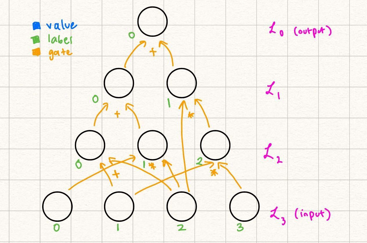
Example
Let's look at the following layered arithmetic circuit with depth = 3:
In this case, and , but . Notice how the circuit naturally falls in "layers" based on the dependencies of values.
Multilinear Extensions (MLEs)
Let be a function . Its multilinear extension is defined such that is linear in each , and where .
Equality MLE
In order to explicitly formulate in terms of , let us define the following indicator function:
Fortunately, has an explicit formula which is linear in each of , or the bits of . Intuitively, if , then each of its bits must be equal. In boolean logic, this is the same thing as saying OR for all of the bits (which is an AND over all of the bits ).
When our inputs this statement can be expressed as the following product: Taking the multilinear extension of simply means allowing for non-binary inputs , because the polynomial is already linear in each variable. Since for all binary we have that , the above definition of is an actual multilinear extension of .
Construction from
We now have a polynomial extension of which happens to be (by construction) linear in the variables (again, denote this function ). We can now define the multilinear extension of any function, as hoped for above:
where are the bits of .
Why is the above a valid multilinear extension of ? The idea here is that when evaluating on any , we have for all (since both and are binary, behaves exactly like the boolean equality function), and thus all the terms in the above summation over are zero except for the term where , where we have , and the value of that term is exactly .
Another nice property of multilinear extensions which can be proven is that they are uniquely defined. I.e., is the only multilinear function in variables which extends .
Example
Let Let us first build a table of evaluations of for
We also build a table for for in terms of :
Then, using the formula for , we get the explicit formula:
.
From here you can verify that when , and that is linear in each of the variables.
Sumcheck
(Most of the content of this section is from Section 4.1 in Proofs, Args, and ZK by Justin Thaler, which has more detailed explanations of the below.)
This section will first cover the background behind the sumcheck protocol, and then provide an introduction as to why this may be useful in verifying the computation of layerwise arithmetic circuits.
The sumcheck protocol is an interactive protocol which verifies claims of the form: In this statement, is not necessarily multilinear, and .
In other words, the prover, , claims that the sum of the evaluations of a function over the boolean hypercube of dimension is Naively, the verifier can verify this statement by evaluating this sum themselves in time assuming oracle access to (being able to query evaluations of in time), with perfect completeness (true claims are always identified by the verifier) and perfect soundness (false claims are always identified by the verifier).
Sumcheck relaxes the perfect soundness to provide a probabilistic protocol which verifies the claim in time with a soundness error of where is the maximum degree of any variable .
The Interactive Protocol
We start with a straw-man interactive protocol which still achieves perfect completeness and soundness in verifier time and prover time Then, we build on this version of the protocol and introduce randomness to achieve verifier time, with a soundness error of
A non-probabilistic protocol
Note that the sum we are trying to verify can be rewritten as such: Let's say sends the following univariate: One way for to communicate to the univariate is to send evaluations of . While can alternatively send coefficients, we focus on this method of defining a univariate and assume sends the evaluations to .
can verify whether is correct in relation to by checking whether In other words, we have reduced the validity of claim that is the sum of the evaluations of over the -dimensional boolean hypercube to the claim that is the univariate polynomial over a smaller sum.
Now the verifier has evaluations to verify. We can similarly reduce this to claims over even smaller summations. Namely, now the prover sends over the following univariates:
and keep engaging in such reductions until is left to verify evaluations of : this is exactly the evaluations of over the boolean hypercube, assuming that has oracle access to (it can query evaluations of in time).
We have transformed the naive solution, where just evaluates the summation on their own, into an interactive protocol. In the next section we will go over how to slightly modify this by adding randomness to significantly reduce the costs incurred by and .
Schwartz-Zippel Lemma
As a brief interlude, let us go over the Schwartz-Zippel Lemma, which we can use to modify the straw-man protocol. It states that if is a nonzero polynomial with degree , then the probability that for some random value sampled from a set is upper-bounded by .
This is can be seen because by the Fundamental Theorem of Alegbra, has at most roots. We take the probability that we randomly sampled one of those roots out of a set of size .
In the case of sumcheck, we consider the polynomial to be over a field , and our randomly sampled element to be uniformly sampled from .
Introducing randomness
Our main blow-up with the straw-man interactive protocol came from the exponentially growing number of claims had to verify, ending up with evaluations of at the end. Instead, if we found a way for the reduction from to claims on (or the reduction from the claim of to claims on ) to be a one-to-one reduction in terms of number of claims, rather than one claim reduced to two claims, would only have to verify claims, and would only have to send over univariate polynomials.
Let us keep the first step the same, where first sends the following univariate polynomial:
Now, checks whether Instead of sending both and , uniformly samples a random challenge from and sends this to sends a single univariate: checks whether This process is repeated iteratively, until finally in the last round, where sends the following:
Assuming the verifier has oracle access to , the verifier can check whether . The difference between this protocol and the naive protocol above is that at each step, instead of individually verifying and , sends a "challenge" in which responds to by sending over the appropriate univariate polynomial. Therefore we have achieved a one-to-one claim reduction, and the verifier having to only verify one equation per round.
Soundness Intuition
We provide brief intuition for the soundness bound from the above protocol. At any step , the prover can cheat by sending a different univariate polynomial instead of the expected such that , but . This allows them to, ultimately, prove a different original statement: that the sum . Because sends to , we can be confident that does not adversarially choose to be one of the roots of . Then, by the Schwartz-Zippel lemma, the probability that happened to be one of the "zeros" of where is the degree of
Example
We do a short example of the sumcheck protocol in the integers. Let rightfully claims that In order to verify this claim, and engage in a sumcheck protocol.
sends the univariate: verifies that Then, samples the challenge and now computes:
checks that Next, samples another challenge and sends it to who then computes and sends Finally, samples another random challenge and checks whether Indeed,
Why Sumcheck?
In the previous section, we introduced the notion of a multilinear extension of a polynomial , which is defined as Notice that naturally, a multilinear extension is defined by taking the sum over a boolean hypercube, which is what sumcheck proves claims over.
In the next section, we will go over how we can encode layers of circuits as multilinear extensions, and prove statements about the output of these layers using sumcheck.
Encoding Layers in GKR
At this point, we have all the puzzle pieces needed to describe the GKR protocol -- layered arithmetic circuits, multilinear extensions, and sumcheck. This section talks about how we can tie all of these concepts together to verify claims on the output of an arithmetic circuit.
Grounding Example
We start with an example layered arithmetic circuit. Throughout this tutorial, we will provide this concrete example while simultaneously providing the generic steps of GKR.
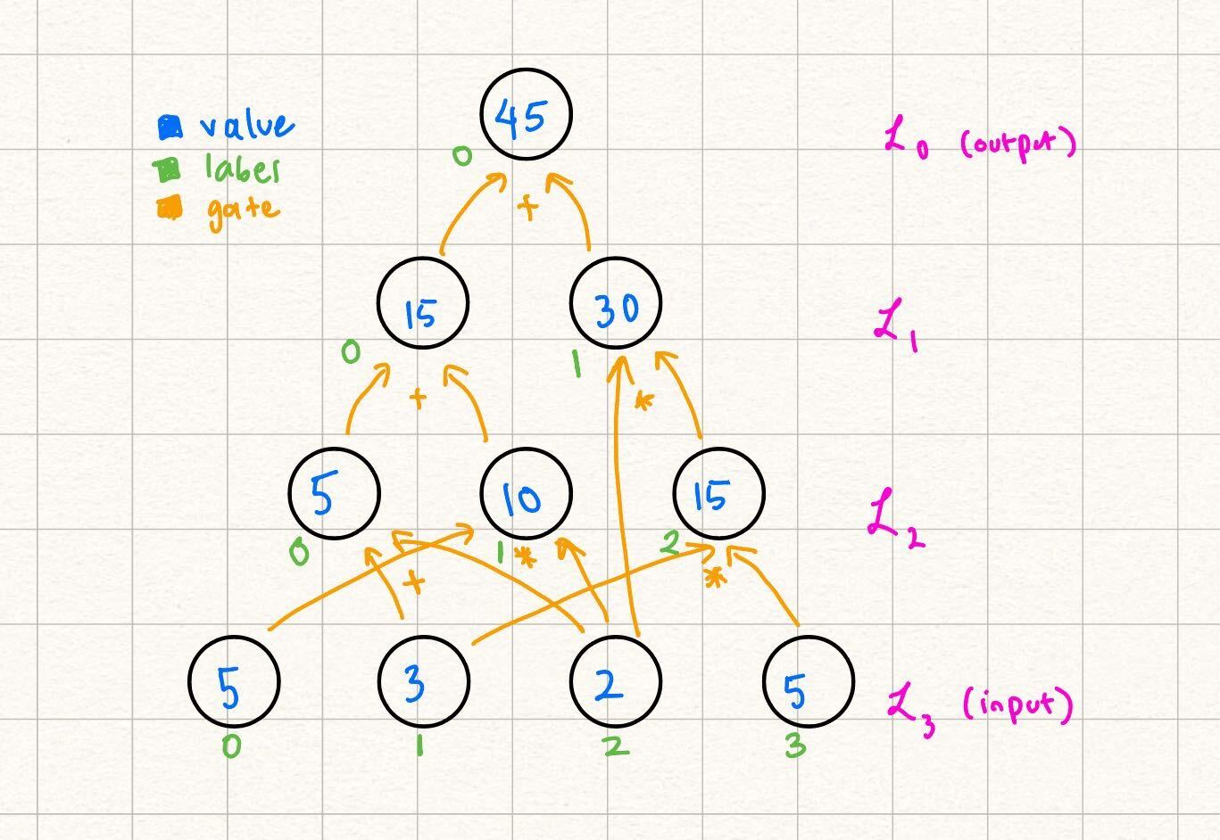
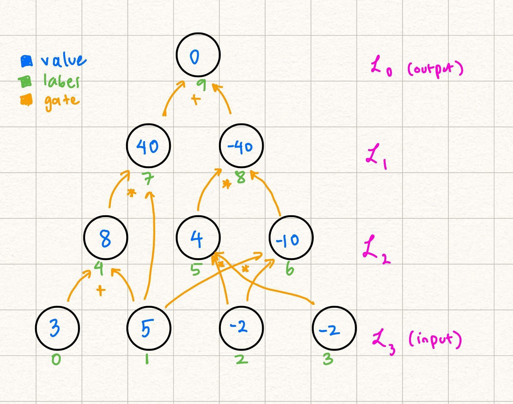
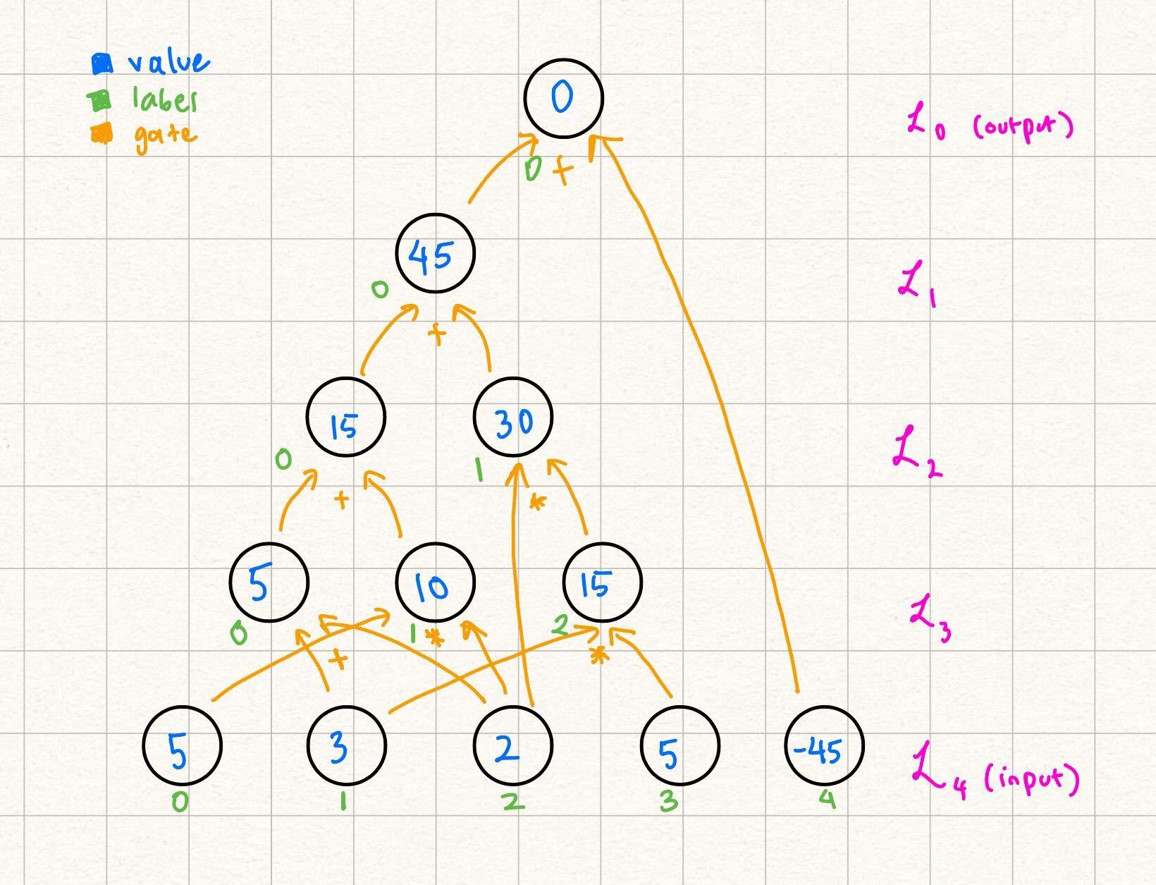
Note some differences from the way this circuit is labeled as opposed to the example in the statement encoding section. Over here, we let the output be a nonzero value for the sake of the example (we explain how to transform any circuit with nonzero output to a circuit with zero output in a future section). Additionally, note that the gate labels start from in each layer, as opposed to the labels being unique throughout the entire circuit in the previous example. Because our gates and are unique per triplet of layers , we can start from in labeling the gates at the start of each layer.
In this example, claims that the output of the following circuit is Note that beyond the values in the input, and the actual structure of the circuit (what we refer to as the circuit description), does not need any more information to verify the output of the circuit by computation:
This is because every node in every layer with can be computed as the result of gates applied to nodes in previous layers.
At a high level, for the rest of this section we focus on encoding layers in two ways: as an MLE of its own, and using its relationship to other layers (via gates). We can equate these two encodings because they are of the same thing (the values in a single layer). With that, we have an equation we can perform a sumcheck over.
Encoding Layer Nodes as an MLE
We start by encoding the input layer in our example, and then show how this extends to the general case. More concretely, we want an MLE such that Although it might not be immediately evident, because we eventually want to invoke the sumcheck protocol, it is useful to consider the inputs as bit-strings rather than integral values.
Example
Therefore, for example, we want because and the bit-string represents . Another way of restating our problem statement of encoding the input layer as some MLE is to say "when , output
Here we can leverage the power of the MLE: or in other words: You can independently verify that at each of the node input label values, outputs the correct value.
General
Note that we conveniently defined the node labels to start from and naturally enumerate the nodes in each layer in our definition of above. This allows us to generally extend the function which represents the nodes of layer into the following MLE: where is the number of nodes in layer .
Encoding Layers using their Relationship to other Layers
Another note we made when presenting the above diagram was that the only information that needs to know immediately is the values of the input itself and the structure of the circuit. This is because the values of the future layers are determined by nodes in previous layers and the gates that connect them. Let's formalize this statement below.
Example
In the running example, let's fill in the layer
We were able to fill this in because:
So, while one way to write the MLE representing , as explained in the previous section, is we can also represent it by its relationship to the nodes in Note that in this definition, we still are linear in the variables
General
Now we go over how to write in terms of for Recall the definition of and . For example, in the case of :
If we use the indicator functions and to translate the example above: where are the number of bits needed to represent the node labels of that respective layer. We know that and can be computed using MLEs for and , so we can rewrite the above as: More detail and examples on transforming these indicator gate functions into MLEs are described in the section on canonic GKR.
Using the Equivalence between Layer Encodings
Now we have enough information to show how we can reduce claims on one layer to claims on the output of an MLE encoding a source layer (closer to the circuit input layer) for that layer.
Example
We start with the MLE encoding the output. claims that the output of the circuit is , i.e., . Then, at any random point challenges with, say , because is a constant function, an honest claims that .
Another way, as expressed above to write is as:
Note that while we expicitly write to maintain consistency between earlier examples, in this case, because there is only one output, there are no variables. Therefore, and are constant functions, and their extensions are equal to their value in their first position: and .
and engage in a sumcheck protocol to verify this claim of the sum of a polynomial over the boolean hypercube. Recall that sumcheck requires binding the variables that the sum is over (in this case, ), one by one, with random challenges.
If we follow the sumcheck protocol as is, at the end, is bound to and is bound to . Let's say the prover's final univariate is and the verifier's final challenge is Then, we end with the final claim:
knows the structure of the circuit, so they can compute on their own. Additionally, is publically computable, so computes that on their own as well. Normally, sumcheck would require make a query to an "oracle" to verify the claimed values and .
However, instead we say that "reduces" the claim that to two claims on
Similarly, has a relationship to MLEs in later layers, so the sumcheck on will reduce to claims on these MLEs, eventually propagating to claims on the input layer.
For another example of claim reduction for structured GKR, see this section.
General
In general, GKR works very similarly to the example above. We cover the case where expects the output of the circuit to be . receives a challenge from and claims that the MLE representing still evaluates to over that random point. I.e., claims that Using the encoding of using later layers, reduces its claim on the output of the circuit to evaluations of MLEs representing future layers.
Note that there is an exponential blow-up of claims when reducing claims on one layer to the next. We describe a protocol to aggregate claims (and therefore achieve a one-to-one reduction) in the claims section.
Circuit Description
Throughout this section, we refer to using the description of the circuit in order to evaluate the gates or to understand the layerwise relationships on their own. The circuit description is something agreed upon beforehand with and and visible to both parties -- it is the "shape" of the circuit, which includes how many nodes each layer contains, the number of layers, and which gates connect nodes from layer to layer.
Therefore, the circuit description of our example circuit is this:
Note: Transforming a Circuit to have Zero Output
In Remainder, expects circuits to have output . This is because certain types of circuits (such as those resulting from LogUp) require the output to specifically be , and needs to specifically verify this fact.
If a circuit does not have output , one way to transform this is to add the negative of the expected output to the input. The last layer of the circuit can be the sum of this expected output, and the actual output of the circuit. This results in a circuit with the output layer evaluating to . We show this transformation applied to our example above:
GKR Theory Overview
Read the introduction and ready to dive into some deeper GKR theory concepts? Let's go!
Structured ("Sector") GKR
Source: Tha13, section 5 ("Time-Optimal Protocols for Circuit Evaluation").
Review: Equality MLE
We begin by briefly recalling the MLE (see this section for more details). We first consider the binary string equality function , where
This function is if and only if and are equal as binary strings, and otherwise. We can extend this to a multilinear extension via the following -- consider , where
Structured Layerwise Relationship
See Tha13, page 25 ("Theorem 1") for a more rigorous treatment. Note that Remainder does not implement Theorem 1 in its entirety, and that many circuits which do fulfill the criteria of Theorem 1 are currently not expressible within Remainder's circuit frontend.
Structured layerwise relationships can loosely be thought of as data relationships where the bits of the index of the "destination" value in the 'th layer are a (optionally subset) permutation of the bits of the index of the "source" value in the 'th layer for . As a concrete example, we consider a layerwise relationship where the destination layer is half the size, and its values are the element-wise products of the two halves of the source layer's values: Let represent the MLE of the destination layer, and let represent the MLE of the source layer.
Let the evaluations of over the hypercube be . Then we wish to create a layerwise relationship such that the evaluations of over the hypercube are . We can actually write this as a simple rule in terms of the (integer) indices of as follows:
If we allow for our arguments to be the binary decomposition of rather than itself, we might have the following relationship:
where is the binary representation of and is the binary representation of . This is in fact very close to the exact form-factor of the polynomial layerwise relationship which we should create between the layers -- we now consider the somewhat un-intuitive relationship
One way to read the above relationship is the following: for any (binary decomposition) , the value of the 'th layer at the index represented by should be . We are summing over all possible values of the hypercube above, , and for each value we check whether the current iterated hypercube value "equals" the argument value. If so, we contribute to the sum and if not, we contribute zero to the sum.
In this way we see for that all of the summed values will be zero except for when are exactly identical to , and thus only the correct value will contribute to the sum (and thus the value of ).
As described, the above relationship looks extremely inefficient in some sense -- why bother summing over all the hypercube values when we already know that all of them will be zero because will evaluate to zero at all values except one?
The answer is that it's not enough to only consider for binary , as our claims will be of the form , where , and is the multilinear extension of (see claims section for more information on prover claims). Another way to see this is that the above relationship is able to be shown for each , but we want to make sure that the relationship holds for all . Rather than checking each index individually, it's much more efficient to check a "random combination" of all values simultaneously by evaluating at a random point . We thus have, instead, that
Since is identical to (and similarly for and ) everywhere on the hypercube, the above relationship should still hold for all binary . Moreover, the above relationship is now one which we can directly apply sumcheck to, since we have a summation over the hypercube!
But wait, you might say. This still seems wasteful -- why are we bothering with this summation and polynomial? Why can't we just have something like
Unfortunately the above relationship cannot work, as are linear on the LHS and quadratic on the RHS. The purpose of the summation and polynomial is to "linearize" the RHS and quite literally turn any high degree polynomial (such as ) into its unique multilinear extension (recall the definition of multilinear extension).
We see that the general pattern of creating a "structured" layerwise relationship is as follows:
- First, write the relationship in terms of the binary indices of values between each layer. In our case, .
- Next, replace on the LHS of the equation with formal variable , and allow the LHS to be a multilinear extension. We now have on the LHS.
- Next, replace on the RHS of the equation with boolean values and add an predicate between , and add a summation over all values. Additionally, extend all to their multilinear extensions (this is importantly only for sumcheck):
Structured "Selector" Variables
Some relationships between layers are best expressed piece-wise. For example, let's say that we have a destination layer, , and a source layer of the same size, , where we'd like to square the first two evaluations but double the last two.
In other words, if has evaluations over the boolean hypercube, then should have evaluations . If we follow our usual protocol for writing the layerwise relationship here, we would have something like the following for the "integer index" version of the relationship:
We notice that in binary form, whenever (and when ). We can thus re-write the above as
In other words, when the second summand on the RHS is zero, and the first summand is just since we already know that , and vice versa for when . At a first glance, this may look similar to the earlier example in which we took the products of adjacent pairs of layer values, but the two are not the same --
- First, the current setup is semantically quite different; in the previous example we applied a binary "shrinking" transformation between the source and destination layers by multiplying pairs of values, while in the current example we are "splitting" the circuit into two semantic halves and applying a different unary operation element-wise to each half.
- Second, the current setup actually has its variable outside of the argument to an MLE representing data in a previous layer. This is precisely what allows us to "select" between the two semantic halves of the circuit and compute an element-wise squaring in the first and a doubling in the second.
Applying the third transformation rule from above and extending everything into its multilinear form, we get
However, now the observation that should only apply to variables which are nonlinear on the RHS is helpful here -- notice that although as a variable would be quadratic on the RHS, is linear and can thus be removed from the summation altogether and replaced directly with :
This layerwise relationship form-factor is called a "selector" in Remainder terminology and in general refers to an in-circuit version of an "if/else" statement where MLEs representing the values of layers can be broken into power-of-two-sized pieces.
Why Structured Circuits?
Compared to canonic GKR, structured circuits are good for two reasons -- verifier runtime and circuit description size. Note that every layerwise relationship which can be expressed as a structured layer (using ) can be written as an equivalent series of and gate layers.
To see why structured layers are good for circuit description size, we compare the following layer-wise relationships which describe the same circuit wiring pattern, but with different verifier cost and circuit description complexities (let and for shorthand). Firstly, the structured version, which computes an element-wise product between each pair of evaluations:
And secondly, the multiplication gate version:
We first consider the verifier runtime for both. Note that the sumcheck verifier performs operations per round of sumcheck, plus the work necessary for the oracle query. In the structured relationship's case, there are rounds of sumcheck, and assuming that get bound to , the oracle query which the verifier must evaluate is of the form
where is the 'th univariate polynomial which the prover sends during sumcheck. The prover sends the claimed values for both and , and so the verifier doesn't do any work there. The verifier additionally evaluates on its own, which it can do in time.
Next, we consider the verifier runtime for the multiplication gate case: let be bound to and let be bound to during sumcheck. The oracle query is then
Similarly to the structured case, the prover sends claimed values for and , and so the verifier doesn't have to do any work here. However, the verifier must also evaluate on its own. This requires time linear to the sparsity of the polynomial, i.e. in this example, since there are nonzero multiplication gates (one for each pair of values in layer ).
A circuit description size comparison between the two can be seen in a very similar light. In particular, the representation of requires just words to store (assuming each word can hold an -bit value), as we simply enumerate the indices between the 's and the 's. On the other hand, storing the sparse representation of required for linear-time proving requires storing all nonzero evaluations, i.e. such indices in the above example (although one might argue that the representation is quite structured and can therefore be further compressed).
A note on claims
The above example (and other similar layerwise relationships) give us a further prover speedup through the structure of the claims which arise from the oracle query during sumcheck. In particular, the claims which the prover makes to the verifier in the structured case are as follows:
These claims can be aggregated with almost no additional cost to the prover and verifier, as the first challenges are identical between the two and the last challenges are precisely a and a . In particular, the verifier can simply sample and have the prover instead show that
On the other hand, the claims generated by the multiplication gate version of the layer above are in the form
These claims have no challenges in common, and can only be aggregated through interpolative or RLC claim aggregation, both of which are significantly more expensive than the above method.
Costs
In general (note that this does not capture all possible structured layer cases, but should be enough to give some intuition on the prover/verifier/proof size costs for most structured layers), let us assume that our layerwise relationship can be expressed in the following manner -- In other words, we have a layerwise relationship over variables, where the values in are a function of those in layers , where , such that we have total summand "groups" of MLEs over variables of size up to , i.e. the total polynomial degree in each of the is .
The prover costs are as follows:
-
For simplicity here, we assume that the prover has access to any value in (note that these evaluations must be either precomputed in linear time, e.g. Tha13, or can be streamed in linear time in a clever way, e.g. Rot24).
-
Additionally, we assume that the prover has access to any value in any , since the prover presumably knows all of the circuit values ahead of time.
-
Finally, we assume that the prover can use the "bookkeeping table folding" trick from Tha13 to compute both from and from in field operations.
-
We thus see that in the first round of sumcheck, the prover must do the following:
- Evaluate each of the terms in the summation for every and sum them together. Each evaluation takes field operations, as there are summands and each requires multiplications.
- Since there are values of , the above costs field operations. This is the total cost for the prover to compute the claimed sum for the first round.
- Next, the prover must evaluate the RHS of the sumchecked equation at in the place of to compute the univariate sumcheck message. Each evaluation of , similarly to the above, costs field operations.
- The total cost for the prover to compute the claimed sum + univariate message in the first round is thus field operations.
-
We can generalize the above to the 'th round of sumcheck (let for the first round) by noting that rather than variables, there are variables which are being summed over in the outer sum. Since the other values remain constant, the prover's total cost is simply .
-
Finally, as mentioned earlier, the prover can generate the necessary precomputed values from the 'th round from those of the 'th round in , as there are MLEs (including the polynomial) which need their bookkeeping tables to be "folded" in .
-
Putting it altogether, the prover's total cost across all sumcheck rounds is thus
-
Since the above is a geometric series in , we have that the prover's total cost across all rounds is simply
The proof size is as follows:
- For each of the rounds of sumcheck, the prover must send over a degree univariate polynomial to the verifier. Additionally, the prover must send the original sum (although this is actually free in GKR since the verifier already has the prover-claimed sum implicitly through the prover's claim from a previous sumcheck's oracle query).
- Finally, the prover must send over each of its claimed values for the at the end of sumcheck. There are at most claims.
- The proof size is thus simply field elements.
The verifier runtime is as follows:
- For each round of sumcheck, let the prover's univariate polynomial message be . The verifier samples a random challenge and checks whether
- Since the verifier can evaluate and in and performs this check for each of the rounds of sumcheck, they can compute all the intermediate checks in .
- During the final oracle query, the verifier must check whether
- The verifier can compute on its own in , and has access to each of the prover-claimed values for . It can thus compute the RHS of the above in .
- The verifier's total runtime is thus
c# Canonic GKR See XZZ+19, ZLW+20 for more details.
"Gate"-style layerwise relationship
Unlike the structured wiring pattern described in the previous section, "gate"-style layerwise relationships allow for an arbitrary wiring pattern between a destination layer and its source layer(s). In general, these layerwise relationships are defined via indicator functions (these function like the function in structured layerwise relationships, but allow for input wires whose indices have no relationship to those of the output wire). Consider, for example, the canonic layerwise GKR equation, which defines the relationship between a previous layer's MLE ( below) and the current layer's MLE ( below): We define three types of gate layers within Remainder, although they are all quite similar in spirit.
Notation
- Let denote the number of variables the MLE representing layer has (in other words, layer of the circuit has values).
- Let be the MLE corresponding to values in the layer of the circuit which is the "destination" of the gate polynomial relationship.
- Let be the MLE corresponding to values in (one) layer of the circuit which is the "source" of the gate polynomial relationship. Note that always.
- Similarly, let be the MLE corresponding to values in (another) layer of the circuit which is a second "source" of the gate polynomial relationship. Note that always.
Identity Gate
Identity gates are defined in the following way: In other words, is if and only if there is a gate from the 'th value in the 'th layer to the 'th value in the 'th layer. These can be thought of as "routing" gates or "copy constraints", as they directly pass a value from one layer to another. The MLE of the identity function above is defined as follows: The polynomial relationship between the "destination" layer 's MLE and the "source" layer 's MLE is as follows: Assuming that gets bound to during sumcheck, this layer produces two claims -- one on and one on . The former can be checked by the verifier directly (since it knows the circuit wiring and uses the definition of above), and the latter is proven by sumcheck over layer .
Example
We start with a "source" MLE over two variables with four evaluations, and wish to obtain a circular-shifted version of the evaluations of this MLE in layer , i.e. .
For example, let's say that the evaluations of are . We wish for those of to be e.g. . To do this, we can list the "nonzero" identity gate indices, i.e. , such that :
- : the zeroth evaluation of layer is equivalent to the first evaluation of layer .
- : the first evaluation of layer is equivalent to the second evaluation of layer .
- : similar reasoning as above.
- : similar reasoning as above.
For all other tuples over binary values we have that .
Costs
Over here, we go through some of the costs for the prover runtime, proof size, and verifier runtime when performing sumcheck over an identity gate layer. In order to provide some intuition, we analyze the costs of a particular example, which may not encapsulate the general example for identity gate layers.
Let us recall the identity gate sumcheck equation: We can rewrite this as: As observed in XZZ+19, we only need to sum over the wirings which are non-zero (i.e., there exists a re-routing from label in layer to label in layer ). Call the set of non-zero wirings as (here, we say that , i.e. a constant number of wires for each input layer and output layer value). We can rewrite the summation as:
The prover cost for sumcheck over an identity gate layer is as follows:
- The prover must first compute the evaluations of . By summing over the non-zero wirings in , XZZ+19 shows us how to compute an MLE with evaluations of this product in time This involves first pre-computing the table of evaluations of using the dynamic-programming algorithm in Tha13, and then appropriately summing over to fold in the evaluations of
- Next, the prover must compute sumcheck messages for the above relationship. The degree of each sumcheck message is , and thus the prover sends evaluations per round of sumcheck. Since we are sumchecking over , there are rounds of sumcheck and thus the prover cost is for the 'th round of sumcheck. The total prover sumcheck cost is thus
- Letting be a constant, the total prover runtime (pre-processing + sumcheck) is
The proof size for sumcheck over identity gate is as follows:
- There are total sumcheck rounds, each with the prover sending over evaluations for a quadratic polynomial. The proof size is thus field elements, plus extra for the final claim on .
The verifier cost for sumcheck over identity gate is as follows:
- The verifier receives sumcheck messages with evaluations each, and each round it must evaluate those quadratic polynomials at a random point. Its runtime is thus with very small constants.
Add Gate
The concepts for addition and multiplication gates are very similar to that of identity gate above. For add gate, we have the binary wiring indicator predicate: Here, we have that if and only if the 'th value in the 'th layer and the 'th value in the 'th layer sum to the 'th value in the 'th layer. The MLE of is similar to that of : and the polynomial relationship is defined very similarly to that of identity gate: Assuming that gets bound to and gets bound to during sumcheck, a claim on this layer results in three total claims: one on (which the verifier can compute from the circuit description and therefore check on its own), one on , and one on .
Example
We start with two "source" MLEs, over two variables with four evaluations each, and wish to add each value in the first with its "complementary value" in the second. The result should be the MLE representing layer , i.e. .
For example, let's say that the evaluations of are and those of are . We wish to add to , to , and so on. Then our "nonzero gate tuples" are as follows:
- : the zeroth value in the 'th layer is equivalent to the sum of the zeroth value in the 'th layer and the third value in the 'th layer.
- : the first value in the 'th layer is equivalent to the sum of the first value in the 'th layer and the second value in the 'th layer.
- : similar reasoning to the above.
- : similar reasoning to the above.
For all other binary tuples we have that , and our resulting MLE's evaluations should be as follows: .
Costs
Over here, we go through some of the costs for the prover runtime, proof size, and verifier runtime when performing sumcheck over an add gate layer. In order to provide some intuition, we analyze the costs of a particular example, which may not encapsulate the general example for add gate layers.
Let us recall the add gate sumcheck equation: We can rewrite this as: As observed in XZZ+19, we only need to sum over the wirings which are non-zero (i.e., there exists a an addition from label in layer and label in layer to label in layer ). Call the set of non-zero wirings as . We can rewrite the summation as:
Mul Gate
Multiplication gate is nearly identical to addition gate. For mul gate, we have the binary wiring indicator predicate: Here, we have that if and only if the the 'th value in the 'th layer equals the product of the 'th value in the 'th layer with the 'th value in the 'th layer. The MLE of is identical to that of : and the polynomial relationship is defined nearly identically to that of gate: Assuming that gets bound to and gets bound to during sumcheck, a claim on this layer results in three total claims: one on (which the verifier can check on its own), one on , and one on .
Example
We start with two "source" MLEs, over two variables with four evaluations each, and wish to accumulate (add up) the product of the 0th and 2nd evaluations with that of the 1st and 3rd evaluations, and place this into the 0th evaluation in the resulting MLE. The result should be the MLE representing layer , i.e. , whose evaluations are all zero except for its 0th evaluation.
For example, let's say that the evaluations of are and those of are . We wish to multiply and , and and and have those be the zeroth evaluation of the resulting MLE, i.e. . We then wish to multiply and , and and and have those be the first evaluation of the resulting MLE, i.e. .
Then our "nonzero gate tuples" are as follows:
- : The zeroth value in the 'th layer multiplied by the first value in the 'th layer contributes to the zeroth value in the 'th layer.
- : The first value in the 'th layer multiplied by the zeroth value in the 'th layer contributes to the zeroth value in the 'th layer.
- : similar reasoning to the above.
- : similar reasoning to the above.
For all other binary tuples we have that , and our resulting MLE's evaluations should be as follows: . Note here for that we are able to add multiple products to each output value in the 'th layer, and that the same is true for both and . In other words, we actually have unlimited addition fan-in and degree-2 multiplication fan-in.
Costs
Over here, we go through some of the costs for the prover runtime, proof size, and verifier runtime when performing sumcheck over a mul gate layer (note that costs for add gate are very similar). In order to provide some intuition, we analyze the costs of a particular example, which may not encapsulate the general example for add gate layers.
Let us recall the mul gate sumcheck equation: We can rewrite this as: As observed in XZZ+19, we only need to sum over the wirings which are non-zero (i.e., there exists a an addition from label in layer and label in layer to label in layer ). Call the set of non-zero wirings as (we assume that there are at most nonzero mul gate values). We can rewrite the summation as:
The prover cost for sumcheck over a mul gate layer is as follows:
- The prover must first compute the evaluations of for where . XZZ+19 splits this pre-processing into two phases (note that proving the gate layer follows the same strategy). First, we precompute (or stream) the values in in .
- Next, we compute the "phase 1" preprocessing, where we sumcheck over the variables. Here, we can directly evaluate while "folding" by summing over the variables. Similarly, in the second phase, when we compute sumcheck messages over and already have evaluations for , we can "fold" by summing over the variables. Both of these preprocessing steps take time.
- After preprocessing, the prover must compute sumcheck messages for the above relationship. Similarly to the preprocessing step above, sumcheck is done in two phases. First, the prover binds the variables, and then it binds the variables. The degree of each sumcheck message is , and thus the prover sends evaluations per round of sumcheck (this is the same for add gate). Since we are sumchecking over and , there are rounds of sumcheck and thus the prover cost is for the 'th round of sumcheck. The total prover sumcheck cost is thus
- Letting be a constant, the total prover runtime (pre-processing + sumcheck) is
The proof size for sumcheck over mul gate layer is as follows:
- There are + total sumcheck rounds, each with the prover sending over evaluations for a quadratic polynomial. The proof size is thus field elements, plus extra for the final claims on and .
The verifier cost for sumcheck over mul gate layer is as follows:
- The verifier receives sumcheck messages with evaluations each, and each round it must evaluate those quadratic polynomials at a random point. Its runtime is thus with very small constants.
GKR Claims
Claim definition
"Claims" in GKR are statements which the prover has yet to show correctness for. As described earlier, the first step in proving the correctness of a GKR circuit (after sending over all circuit inputs, both public and committed) is to take the circuit's (public) output layer and send over all of its evaluations to the verifier.
For example, let's say that we have a circuit whose output layer contains 4 elements, i.e. whose representative MLE can be described by . Additionally, let's say that these evaluations are , such that
These four equalities above are actually the first claims whose validity the prover wishes to demonstrate to the verifier. The verifier doesn't know what the true values of are, of course, but would be able to check each of these relationships with the prover's help via sumcheck. This would be rather expensive, however, as the number of claims is exactly equal to the number of circuit outputs/evaluations within the circuit's output layer. Instead, the verifier can sample some randomness and have the prover prove the following:
Note that the above follows precisely from the definition of a multilinear extension (MLE), and it can indeed be viewed exactly as the evaluation of at the random points . The protocol takes a slight soundness hit here, as a cheating prover might get away with an incorrect circuit output (say, , but ), but the probability of such an occurrence is , as non-identical MLEs only intersect at exactly one point via the Schwartz-Zippel lemma.
In general, claims take the following form:
In other words, the prover wishes to convince the verifier that the evaluation of the MLE representing the 'th layer at the challenge is .
Claim Propagation
For another example of claim propagation/reduction, see this section. Note that the below example uses a structured GKR relationship while the other example uses a canonic GKR relationship.
Recall the general sumcheck relationship for a function ; the prover claims that the following relationship is true for :
Assuming that are bound to during the sumcheck process, the final verifier check within sumcheck is the following, where the RHS must be an "oracle query", i.e. the verifier must know that the evaluation of on is correct:
How does this oracle query actually get evaluated in GKR? The answer is claims and sumcheck over claims for a previous layer. Specifically, let's consider the following relationship (see structured GKR section for more information about the polynomial and this kind of layerwise relationship):
This is the polynomial relationship between layer and layer of a circuit where the 'th layer's values are exactly those of the 'th layer's values squared. For example, if the evaluations of are then we expect the evaluations of to be .
The prover starts with a claim
for , and wishes to prove it to the verifier. It does so by running sumcheck on the RHS of the above equation, i.e.
Let be bound to during the rounds of sumcheck. Additionally, let be the univariate polynomial the prover sends in the 'th round of sumcheck. The oracle query check is then
The verifier is able to compute on its own in time, but unless is an MLE within an input layer of the GKR circuit, they will not be able to determine the value of . Instead, the prover sends over a new claimed value , and the verifier checks that
The only thing left to check is whether . Notice, however, that this now a new claim on an MLE residing in layer , and that we started with a claim on layer . In other words, we've reduced the validity of a claim on layer to that of a claim on layer , which is the core idea behind GKR: start with claims on circuit output layers, and reduce those using sumcheck to claims on earlier layers of the circuit. Eventually all remaining claims will be those on circuit input layers, which can be directly checked via either a direct verifier MLE evaluation for public input layers, or a PCS evaluation proof for committed input layers.
Claim Aggregation
In the above example, we reduced a single claim on layer to claim(s) on MLEs residing in previous layers. What happens when there are multiple claims on the same layer, e.g.
One method would be to simply run sumcheck times, once for each of the above claims, and reduce to separate claims on MLEs residing in previous layers. This strategy, however, leads to an exponential number of claims in the depth of the circuit, which is undesirable.
Instead, Remainder implements two primary modes of claim aggregation, i.e. methods for using a single sumcheck to prove the validity of many claims on the same MLE.
RLC (Random Linear Combination) Claim Aggregation
Additional reading: See XZZ+19, page 10 ("Combining two claims: random linear combination").
The idea behind RLC claim aggregation is precisely what it sounds like: the prover shows that a random linear combination of the claimed values indeed equals the corresponding random linear combination of the summations on the RHS of e.g. the third equation in the above section. The implementation of RLC claim aggregation within Remainder works for structured layers and gate layers, but not for matrix multiplication layers or input layers (as explained below).
We defer to the corresponding pages for more detailed explanations of the layerwise relationships, but review their form factors here and show how RLC claim aggregation can be done for each here.
Structured Layers
We start with structured layers, and use the same example relationship from above:
For simplicity, we aggregate two claims rather than claims, but the methodology generalizes in a straightforward fashion. Our aggregated claim is constructed as follows:
Similarly, we take an RLC of the summations and create a new summation to sumcheck over (we let and for concision):
For structured layers, in other words, the prover and verifier simply take a random linear combination of the claims and perform sumcheck over a polynomial which is identical to the original layerwise relationship polynomial but with the term replaced with an RLC of terms in the same manner as the RLC of the original claims.
Gate Layers
A similar idea applies to gate layers. We use mul gate as the example layerwise relationship here:
Again, we aggregate just two claims for simplicity, although the idea generalizes very naturally to claims:
The polynomial relationship to run sumcheck over is constructed using a similar idea as that of structured layers:
Rather than taking a linear combination of the polynomials, we instead take a linear combination of the polynomials.
Costs
The prover costs for RLC claim aggregation are as follows -- assume that we are working with a structured layer (the analysis is similar for gate layers) and that the degree of every sumcheck variable is (in the above example for a structured layer, ). Additionally, assume that we have claims over a layer with variables.
- As shown above, RLC claim aggregation for structured layers simply involves "factoring out" the term between each of the 's and the 's. Rather than multiplying the structured polynomial relationship by a single , we multiply by an RLC of terms.
- For each additional term, the prover incurs an additional evaluations worth of work (across a single sumcheck round). Evaluating can be done in time by the prover for variables, and thus the total cost (for claims) is
- across all rounds of sumcheck. The total prover runtime is thus .
The proof size is identical to that of the single-claim sumcheck case, since the degree of the sumcheck messages do not change.
Finally, the verifier cost is slightly increased. Specifically, during intermediate rounds of sumcheck the verifier does not do any additional work (compared to the single-claim sumcheck case), but during the oracle query the verifier must evaluate separate instances of at fixed points. This takes the verifier additional time.
Matrix Multiplication Layers (counterexample)
Prerequisite: matrix multiplication layers page.
For matrix multiplication layers: consider , and consider the sumcheck relationship .
In matrix multiplication layers, the claim is always of the form , and the prover proceeds by first binding and before showing that . In the RLC claim aggregation case, we have claims Where and (otherwise they would be claims from the same "source" layer and would therefore be identical). The verifier samples random challenge . In this case, our sumcheck relationship is the following: Because and , there is no way to factor the above expression's RHS to combine terms in any way, and thus RLC claim aggregation is equivalent to not aggregating claims at all and simply running two separate sumchecks on
Input Layers (counterexample)
For input layers: RLC claim aggregation combines claims into a single claimed statement For public inputs, the verifier must evaluate each of and on their own, and thus nothing is gained by the combination.
For committed inputs, a polynomial commitment scheme may allow for cheaper evaluation proofs in the above form (vs. two separate evaluation proofs; one for each claim), but this is generally not the case.
Interpolative Claim Aggregation
Additional reading: See Tha13, page 15 ("reducing to verification of a single point"), for another description of the protocol, and Mod24, page 15 (Section 3.4, "Claim aggregation"), for a thorough description + optimization.
Interpolative claim aggreation works by having the prover and verifier both compute an interpolating polynomial , such that for the claims described earlier, i.e.
we have that
Note that the degree of is , as there are points for each of the coordinates which must be interpolated.
The prover then sends over the polynomial , i.e. the restriction of to points in generated by . Note that the degree of is , as is multilinear in each of its variables, and each of those variables is degree at most in the input variable for .
The verifier samples and sends it to the prover. The prover and verifier both compute , and the prover proves the single claim
where was sent by the prover and the verifier evaluates it at on its own.
Costs
The prover cost for interpolative claim aggregation is as follows:
- Given claims with variables each, is a -degree function in each of its components, and since is multilinear in each of its variables, is a univariate polynomial with degree . The prover must send evaluations to the verifier, although the first have already been sent implicitly in the form of the claims.
- The prover thus must evaluate at points. Each evaluation requires the prover to evaluate in time, and then in time. The prover's total runtime is thus .
The proof size for interpolative claim aggregation is as follows:
- As reasoned earlier in the prover cost section, the prover sends over evaluations of . The proof size is thus field elements.
The verifier runtime for interpolative claim aggregation is as follows:
- The verifier receives evaluations of from the prover and evaluates it at a random point . This takes time. Additionally, the verifier evaluates , which takes time as well. The verifier's total runtime is thus .
Optimizations
Remainder has a few built-in optimizations for interpolative claim aggregation which substantially lower the prover costs for claims with "structure" within their evaluation points. For more details, see Mod24, page 15 (Claim Aggregation section).
Matrix Multiplication Layer
A GKR "matrix multiplication" layer is one which takes as input two MLEs and outputs a single MLE whose evaluations are the flattened matrix multiplication of the evaluations of and .
Canonic matrix multiplication is defined as the following, given matrices resulting in :
where the above holds for , . We instead consider the multilinear extensions of the above matrices, such that
where . Then for all and we have
(Note that the above is also necessarily true for general , as multilinear extensions are uniquely defined by their evaluations over the boolean hypercube.) We wish to prove this relationship to the verifier using sumcheck. We can do this using Schwarz-Zippel against as follows: rather than checking the above relationship for all , the verifier can sample challenges and instead check the following relationship:
This is a sumcheck over just variables, and yields two claims (assume that is bound to during sumcheck) –
Costs
The prover cost for sumcheck over matrix multiplication is as follows:
- The prover must first compute the evaluations of and for . It already has the evaluations of and , and thus this preprocessing step takes .
- Next, the prover must compute sumcheck messages for the above relationship. The degree of each sumcheck message is , and thus the prover sends evaluations per round of sumcheck. Since we are sumchecking over , there are rounds of sumcheck and thus the prover cost is for the 'th round of sumcheck. The total prover sumcheck cost is thus
- The prover's total cost (preprocessing + sumcheck) is . Letting be a constant and allowing square matrices with , the prover's total cost is , which is asymptotically optimal for matrix multiplication.
The proof size for sumcheck over matrix multiplication is as follows:
- There are total sumcheck rounds, each with the prover sending over evaluations for a quadratic polynomial. The proof size is thus field elements, plus extra for the final claims on and .
The verifier cost for sumcheck over matrix multiplication is as follows:
- The verifier receives sumcheck messages with evaluations each, and each round it must evaluate those quadratic polynomials at a random point. Its runtime is thus with very small constants.
GKR Input Layer
We have now seen that a GKR interactive proof begins with the prover making a claim on the layered circuit's output layer and reducing this claim via sumcheck and claim aggregation to claims on layers closer to the circuit's input layer, e.g. .
At the end of this process, we should be left with only claims on input layer(s), e.g.
These claims are optionally aggregated via interpolative claim aggregation (note that RLC claim aggregation does not work for input layer claims; see here for more details) into a single claim
which the verifier must check on its own, optionally with help from the prover. There are several types of input layers, and we describe the methodology for each.
Public Inputs
Public input layers are circuit inputs where the prover sends the values to the verifier in the clear. In particular, this means that the verifier knows the full set of evaluations of over and can evaluate the MLE on its own. Thus:
- Before the prover generates the output layer claim challenges ( above), they send these evaluations to the verifier by absorbing them into the transcript.
- When the verifier is ready to check the claim , they use the aforementioned evaluations to directly evaluate at and check that the evaluation is indeed the claimed .
Committed Inputs
Committed input layers are circuit inputs where the prover sends a commitment to the values (generally as a polynomial commitment). Committed inputs are not directly revealed to the verifier (although they may leak information unless a zero-knowledge polynomial commitment scheme, like Hyrax, is used), and thus the prover must additionally help the verifier when they wish to check the input claim by providing an evaluation proof, which roughly shows that the polynomial which the prover committed to earlier actually evaluates to at the evaluation point .
(See KZG10, page 6, and Tha24, page 188 for more details). Let be the security parameter. Let be the MLE which the prover wishes to commit to. Let be the evaluation point, and let be the claimed value. Roughly speaking, a polynomial commitment scheme (PCS) consists of the following four functions:
- . here is the commitment key which the prover has access to while committing and generating evaluation proofs, and here is the verification key which the verifier has access to while checking an evaluation proof. This function takes in a single security parameter such that the resulting commitment scheme has roughly bits of soundness.
- . The function takes in an MLE (for our purposes; in general this can be a univariate or multivariate polynomial of higher degree) and generates a commitment to be sent to the verifier.
- . The function takes in an evaluation point and produces an evaluation proof that the original polynomial which was committed to in actually evaluates to . Note that the verifier uses to check the evaluation proof .
- . The function takes in a commitment and an MLE and outputs whether that MLE is the one committed to by , i.e. whether .
In addition to the above, a commitment scheme must satisfy hiding and evaluation binding.
- Hiding implies that given a commitment and fewer than evaluation pairs, an adversary cannot determine the evaluation for a point not in the set of evaluation pairs.
- Evaluation binding implies that given an evaluation point and a claimed value , a prover should be able to produce an accepting evaluation proof for generated with negligible probability.
In general, we run once and distribute the resulting to the prover and verifier, and focus on the and functions. During the interactive GKR protocol, the prover and verifier do the following:
- The prover invokes the functionality on and sends the resulting to the verifier. They send this value to the verifier before any claims on output layers (including challenges) are generated. Note that this takes the place of the prover sending the evaluations of in the public inputs section above.
- After the prover has sent all circuit inputs to the verifier in either committed or direct evaluation form, the verifier generates the output claim challenges and the prover and verifier engage in the GKR claim reduction protocols until we're left with a single claim .
- The prover then invokes the functionality on and the aforementioned values to produce evaluation proof , which the verifier receives and checks.
Remainder's GKR prover uses a non-ZK version of the PCS implicit in AHIV17 (also explicitly described in the GLS+21 paper as Shockwave), which we briefly detail in our documentation's Ligero PCS page. Remainder's Hyrax prover uses the ZK PCS explicitly described within WTS+17, which we briefly detail in our documentation's Hyrax PCS page.
"Fiat-Shamir" Inputs
A third type of circuit "input" is that of a "Fiat-Shamir" challenge value. These inputs are different from the others in the sense that the prover does not supply them at all, but rather the (interactive) verifier sends them after the prover has committed to all other input values. These values are used when the circuit itself is computing a function which requires a random challenge (see LogUp, e.g., for one usage of such challenges). In general, claims on these layers are checked via the following:
- First, as mentioned, the (interactive) prover sends all other inputs (both public and committed) to the verifier.
- Next, the verifier sends random values (we can view these as the evaluations of over ) to the prover as challenge values.
- When the verifier needs to check a claim on the Fiat-Shamir input layer, it can do so by simply referencing the evaluations it generated earlier to evaluate at and ensure that the evaluation is actually , exactly as is the case for public inputs.
Ligero Polynomial Commitment Scheme
References: GLS+21, page 46, AER24.
Prerequisites
As described within the committed input layers section, the Ligero polynomial commitment scheme (PCS) consists of a and an phase such that
- During , the prover sends a commitment for the input layer MLE .
- After running the rest of the GKR claim reduction process, we are left with a claim .
- During , the prover sends an evaluation proof showing that .
Short Introduction to Reed-Solomon Codes
We provide a brief introduction to Reed-Solomon codes, as these are prominently featured within the Ligero construction. First, we describe a few properties of general linear codes which will be useful:
- An -linear code is a subspace of dimension (i.e. is spanned by linearly independent basis vectors of length each) where implies that for all nonzero codewords .
- We define the Hamming weight is the number of nonzero entries in .
- For all distinct we have that , since the difference of two codewords is itself a codeword.
- The encoding step of a linear code can be described by a matrix-vector multiplication , where is the unencoded message and is the code's generator matrix. For simplicity we will just use as the encode function notation.
- We call the rate of the code, as it describes (the inverse of) how much redundancy the code has. is then the "expansion factor", or how much larger the codeword is than the original message.
Next, consider the set of (univariate) polynomials of degree and a domain . Let .
- Let be the restriction of to . Note that can be treated as just a vector of length by taking its evaluations .
- We define a Reed-Solomon code , i.e. all the restrictions of to evaluations over for degree functions .
- If we let and call the evaluation domain size , then an RS code is just an linear code (codewords are the evaluations of over , and the un-encoded messages are just polynomials of degree , which can be specified with coefficients).
- Note that two polynomials of degree agree on at most points, and thus the Hamming distance between codewords is .
The last property of Reed-Solomon codes is extremely useful for the purposes of code-based PCSs such as Ligero and FRI -- if we have that , for example, then for two polynomials where we have that , which is over half of the evaluation domain. This intuitively makes it very easy for a verifier to catch a prover who commits to one polynomial's codeword and attempts to evaluate using another's, since sampling even a single random point within will reveal the difference with probability .
Vector-Matrix-Vector Product Observation
(Reader's note: the construction described here is identical to that in the Hyrax PCS section.) Let our input layer MLE have evaluations over (for example, ).
As described in the introduction above, the prover is trying to show that . As described in the Hyrax PCS section, one way to compute the evaluation is as follows:
The column vector on the right can be viewed as the tensor product and we will use this shorthand going forward. Just this observation, however, is not enough to motivate our description of Ligero PCS. Instead, we consider an alternative formulation for the evaluation .
Rather than simply linearly arranging the coefficients of as above, we can instead arrange them in a square matrix (for now, assume that is even) of size by enumerating the coefficients in row-major order:
Given the matrix formulation of above, we can write the evaluation of as the following vector-matrix-vector product:
We denote the left vector as and the right vector as . This allows us to create the following PCS:
Commitment Phase
The commitment phase of Ligero works as follows:
Let be the 'th row of , . Recall that since is a square matrix.
- First, the prover treats the values within as the (monomial basis, i.e. usual) coefficients of a degree- univariate polynomial. They compute using a Reed-Solomon encoding function. Let be the code rate; we then have that .
- The encoded matrix now looks like the following:
The prover commits to as follows:
- Using a cryptographic hash function , the prover first computes a hash over each column:
- Next, the prover takes the vector of column-wise commitments and computes a Merkle tree using those commitments as the leaves. In other words, the bottom layer of the tree is , with pairs of leaves being hashed, and the root of the tree is the commitment.
- The (interactive) prover sends to the verifier. Note that with this commitment setup, the verifier is able to "open" any column of and ensure that it is consistent with the commitment .
Evaluation Phase
The prover wishes to show that . It does so by first computing and sends this to the (interactive) verifier (note that the prover is sending product of against the unencoded ). Since the verifier doesn't (yet) trust this value, we'll denote its view of this prover message as .
The verifier asserts that . If the prover is honest and then this proves that the evaluation was correct.
The verifier then computes , with . To ensure that the prover computed correctly, it will check random values in against .
- Note that because is a linear operation, we have that , where is the row-wise encoding as described earlier (check this for yourself -- use the intuition that Reed-Solomon encoding is just polynomial evaluation over a domain)
The verifier picks a set of indices and "opens" those columns of . For each , the prover sends over , as well as a Merkle path for against .
The verifier checks that , and verifies the Merkle path from to the it received during the commit phase.
The verifier is now convinced that the columns which the prover sent over are columns of the which was committed to during the commitment phase.
Finally, the verifier checks that . This last check ensures that the prover sent honestly -- if they attempted to cheat by sending for some , we have that each row of would differ from each row of in at least proportion of coordinates (as mentioned earlier, we generally have ), and therefore WHP (using a result from AER24), that (the honest ) differs from (the dishonest ) in at least proportion of coordinates as well.
With queries, the verifier catches a cheating prover at least
proportion of the time. We set such that the above probability is at least , where is our security parameter.
Costs
Assume that the prover is committing to a multilinear polynomial in variables. Let our code rate be , and assume that a Reed-Solomon encoding for a message with coefficients to a codeword with evaluations can be computed in time . Let be the set of columns we query during the evaluation phase.
Prover Cost
- During the commitment phase, the prover first computes the encoded matrix of coefficients by encoding each row of . There are rows and each row's encoding takes time for a total runtime of .
- Next, the prover computes hashes of the columns of , and then constructs a Merkle tree comprised of those for the final commitment. This costs hashes.
- During the evaluation phase, the prover first computes and sends the result to the verifier. This takes operations.
- Next, the prover sends over columns plus associated Merkle proofs to the verifier. The prover doesn't need to compute anything here, so this is free for the prover.
- Assuming the cost of a single hash is , the total prover computation is
Proof Size
- The commitment is a single Merkle root, and is thus just one field element.
- The evaluation proof consists of the following for each column :
- A column of with field elements
- A Merkle path with field elements
- Thus the total proof size is field elements.
Verifier Cost
- During the commitment phase, the verifier receives a single Merkle root element and does nothing else.
- During the evaluation phase, the verifier first receives the prover's claimed and computes . The encoding step takes field operations.
- Next, the verifier computes and checks this against the claimed evaluation value. This requires field operations.
- Next, the verifier receives columns of from the prover. For each column, the verifier must
- Compute a hash over elements to get the column hash value.
- Check the Merkle proof over a path of length against the root received in the commit phase.
- The verifier's runtime for the check phase is hashes.
- The verifier's total runtime is
What is a lookup argument?
A lookup argument demonstrates that a given multiset of values (the "witness") contains only values from a prescribed set (the "lookup table").
Common applications of lookup arguments
Lookup arguments find various applications. For example, in a "range check", the values of the witness are constrained to belong to a contiguous range of values. This is useful when a purported digital decomposition in base is provided to the circuit as input, and it is therefore necessary, in particular, to check that the digits are indeed in the range . The lookup table in this case is just this range.
Another example that occurs in the context of machine learning is checking the computation of an arbitrary function (e.g. a non-linearity like the sigmoid) in circuit. Conceptually, in this application the lookup table consists of all valid input-output pairs , and the witness consists of those pairs that are used. Circuits work only with individual field elements, so a random linear combination of the input and output of each input-output pair is formed, i.e. where is a challenge provided by the verifier. When a lookup is used to encode a function in this way, it is referred to as an "indexed lookup" (whereas a range check is an example of an "unindexed lookup").
Naive lookups and their limits
Certain lookups can be implemented in circuit in a direct and elementary fashion. For example, to perform a range check for purported binary digits, it is sufficient to check that the polynomial vanishes for all the digits. This of course generalizes to higher bases. However, this solution is inefficient for large (e.g. >16) bases. In such cases, and also for typical applications of indexed lookups, a more sophisticated lookup argument is significantly more efficient. To this end, Remainder implements the LogUp lookup argument of Papini and Haböck.
LogUp
(We describe only the outline of LogUp. If interested in further details, see here.)
Let denote an MLE of witness values (with variables) and let denote the MLE of table values (with values). For example, when performing a range check on purported base 256 digits, the entries of are the purported digits, while contains the values 0 .. 255 (and ). LogUp additionally involves some auxilliary information in the form of the multiplicities . This MLE has the same length as the table , and specifies the number of times that each table element occurs in the witness. To continue the example, if , then with all other entries being zero. The multiplicities , like the table values , are not computed in circuit, but rather provided as inputs.
LogUp demonstrates that the following equality holds in the field of fractions: Under the assumption that the table values are distinct, this equality is equivalent to the statement: "the entries of contain only entries of , and the value occurs in with multiplicity ".
This equality can be checked using a specialized GKR circuit that is implemented in Remainder. In addition to , this circuit also takes in a challenge provided by the verifier (that is substituted in place of the indeterminate).
Important note on soundness
The implementation of LogUp in Remainder assumes that the field size is significantly larger than the table size and the witness size, and moreover that the witness length is less than the characteristic of the field. These assumptions will always hold for practical tables and witness in the current implementation of Remainder, since it uses the scalar field of the BN254 curve. It should be noted, however, that if Remainder were to be adapted to "small" fields (e.g. 32 bit fields) then soundness problems will arise for large tables and witnesses.
Fiat-Shamir: Creating Non-interactive GKR proofs
As described earlier, both sumcheck and GKR are interactive proofs with many rounds of messages exchanged between a prover and a verifier. However, Remainder is built as a non-interactive proof system, where the transformation we apply is the Fiat-Shamir heuristic, with every prover message being "absorbed" into the state of a hash function with a sponge mode (Poseidon instantiated over the BN-254 scalar field, in our case) and every verifier message being "squeezed" from that same hash sponge.
We note that both sumcheck and GKR have been proven round-by-round sound, i.e. despite being a non-constant-round interactive protocol, can still achieve soundness in the random oracle model when instantiated with a hash function believed to be indistinguishable from a random oracle.
Sponge Functions as Random Oracles
The sponge construction transforms a fixed-length input, fixed-length output permutation function into a variable-length input, variable-length output function which can be shown to behave indistinguishably from a random oracle given that the fixed-length permutation function itself is indistinguishable from an ideal random permutation. As mentioned earlier, Remainder uses the Poseidon sponge (i.e. a standard sponge construction instantiated over the Poseidon fixed-length permutation), and since we assume that the Poseidon permutation is indeed indistinguishable from an ideal random permutation, we only require security in the random oracle model.
Fiat-Shamir for Sumcheck
We describe the Fiat-Shamir transformation for the sumcheck sub-protocol as an example. As before, let be the statement over which we are running sumcheck, i.e. the prover claims that is the sum for a multi-variate polynomial , and the verifier wishes to check this. Recall that in the interactive version of sumcheck, the prover first computes the univariate function
and sends its coefficients to the verifier. The verifier then samples a random challenge and sends this back to the prover. Let be the sponge function instantiation for the random oracle. The prover instead invokes the following:
where and invoke the corresponding sponge functionality over . The rest of the sumcheck rounds proceed in a similar fashion. In the 'th round, the prover computes
and invokes the sponge function via
after receiving , in the interactive version of the protocol the prover would then send the claim to the verifier. Instead, we again call on this value:
In other words, whenever the prover sends a message to the verifier in the interactive version of the protocol, they instead that message into the sponge function, and whenever the verifier sends a challenge to the prover in the interactive protocol, the prover instead calls on the sponge function to sample the challenge instead.
Proof/Transcript
Please read the Fiat-Shamir documentation page before this one!
Transcript
A Remainder Transcript consists of all of the explicit sponge function operations which take place during the generation of a non-interactive (GKR) proof. As mentioned in the Fiat-Shamir documentation page, the prover can interact with the sponge function in two primary ways, exactly corresponding with the interactive version of the protocol:
- When the prover would send a message to the verifier in the interactive version of the protocol, they instead invoke .
- When the verifier would send a challenge to the prover in the interactive version of the protocol, the prover instead invokes .
Remainder's TranscriptSponge captures exactly these operations. You will generally work with the TranscriptWriter and TranscriptReader structs. The TranscriptWriter is the prover's view of the transcript, and the prover can add Operations to the internal Transcript struct. When the prover is finished appending all of their messages (and squeezing challenges where appropriate) to/from the TranscriptWriter struct, they can then eject the internal Transcript and send this directly to the verifier (e.g. as bytes), as the Transcript includes all of the proof data and can be treated as the GKR proof itself (note that this is slightly different from the structured proof within Hyrax). The verifier can feed this struct into the constructor of a TranscriptReader (again, mostly a convenience wrapper around a Transcript for the verifier to read prover messages from and sample Fiat-Shamir challenges from while maintaining its own hash function's sponge state) and consume the Operations in the same order to perform verification.
Appending Input Elements
See append_input_elements() for more details. There is a special function for appending input elements (i.e. all elements which the prover needs to communicate to the verifier before the first output claim challenge is generated), ProverTranscript::append_input_elements(), which should be called. This function provides some insurance against the attack on non-interactive GKR described in this paper by creating a long hash chain (1000 iterations of SHA-256, specifically) for each input -- in general, this prevents most circuits (due to their limited depth) from being able to generate the hash chain value themselves and thus carry out the attack. In general, however, we emphasize that all circuits used in production should be audited to mitigate such attack potential.
Frontend Components
The basic component of a GKR circuit is a layer. A layer is defined as an MLE plus polynomial relationship which explicitly states how each evaluation of that MLE (over the boolean hypercube) is related to evaluations of MLEs within previous layers.
Remainder Components Overview
The layer types which are supported in GKR are as follows:
- "Structured" layers, which define the regular-wiring layerwise relationships described in the "structured GKR" section.
- "Gate" layers, which define the arbitrary-wiring layerwise relationships described in the "canonic GKR" section.
- "Matmult" layers, which define the matrix multiplication-like layerwise relationships described in the "matmult" section.
- "Lookup" layers, which define the lookup (LogUp) arguments described in the "lookup" section.
Additionally, we provide an example of how to compile into a Hyrax-provable circuit rather than a GKR-provable one in this section.
Remainder Circuit Definition
Circuits in Remainder are created via a "compilation" process. In essence:
- Circuit writers (that's you!) define the layer types and layer-wise
relationships by defining
Nodes of the variety as described above. - Circuit writers (still you!) also define the input layers and "shred"s within each input layer for the circuit.
- Additionally, each type of
Noderequires as input references to otherNodes which act as he "source data" for that node's outputs. The data type used in Remainder for storing those references is aNodeRef<F>. The circuit builder returns such references every time a new node is added to the circuit. - Once all of these relationships have been defined, Remainder will compile the set of nodes + source relationships into a layered circuit which can be run and proven/verified. Note that there are a couple of compilation options here, including compiling into the shallowest possible circuit by "combining" layers which are topologically oblivious (i.e. any layerwise ordering is valid).
Sector Layer Frontend Tutorial
To express structured layer-wise relationships in Remainder, we can use a Structured GKR Layer,
a.k.a "Sector" layer. A Sector layer is defined through an AbstractExpression<F> type, also
simply called "Expression" in this tutorial. Expressions can be built by combining MLEs. To refer
to an MLE we use the NodeRef<F> values returned by the circuit builder when the respective MLE was
added. MLEs can be combined through overloaded binary operators (currently available are +, -, *
for addition, subtraction and multiplication respectively), or using a Selector.
Let's walk through a few examples of the usage of Sector layers using Remainder circuit building interface.
Example 1: Multiplying two MLEs
We start with a simple circuit that multiplies two MLEs element-wise: an MLE with evaluations (over the boolean hypercube) with an MLE with evaluations , to produce the MLE with evaluations .
To express this in Remainder, we can simply write:
#![allow(unused)]
fn main() {
/* ... define the input layer `input_layer` ... */

// Define the input shreds for `V_1` and `V_2`.
let v1 = builder.add_input_shred("MLE 1", 2, &input_layer);
let v2 = builder.add_input_shred("MLE 2", 2, &input_layer);

// Define the Sector layer that performs the multiplication operation.
let v3 = builder.add_sector(v1 * v2);
}
In this example the input MLEs to the Sector were input shreds, but in general they can be any node appearing in the circuit. We can, for example, follow the above code segment with:
#![allow(unused)]
fn main() {
let v4 = builder.add_sector(&v3 * &v3);
}
which squares the entries of the MLE .
Implmentation Note: The reason we're borrowing v3 is an unfortunate quirk of the way
the NodeRef<F> type is implemented. It is a wrapper around a weak pointer, and thus not
Copy-able. This means that the multiplication operator will try to take ownership of its two
operands, and after the first occurance of v3 has moved, the second one will fail with a compile
error. To avoid unneseccary cloning, we provide an implementation of the Mul trait for borrowed
operands as well (e.g. &NodeRef<F>) to allow developers to use the succinct borrowed syntax
we presented above when there is a need to reuse NodeRef<F>s.
Expressions may be combined into a single Sector layer. For example, previously we expressed the relation using two layers, but we could have equivalently written:
#![allow(unused)]
fn main() {
let v4 = builder.add_sector( (&v1 * &v2) * (&v1 * &v2) );
}
See run_example_1a() in
frontend/examples/sector.rs
for the full code of the preceeding examples.
Efficiency Note: It's important to note that the two alternative ways of defining v4
presented above result in different circuits, even though they're semantically equivalent. The
circuit's structure (number of layers, expression structure etc.) can affect the prover/verifier
runtime. Refer to Section 3: GKR Theory for more information.
What would happen if we tried to multiple two MLEs of different sizes? You might expect that element-wise operations are not well defined if the two MLEs are not of the same size, but there is a mathematically natural interpretation for such a formula, which we adopt in Remainder.
Let be an MLE on two variables, and be an MLE on only one variable. One natural interpretation for the expression is an MLE on two variables defined by , i.e. equating the common MLE variables starting from the left.
Viewing the MLEs as evaluation vectors, if and , then .
See run_example_1b() in
frontend/examples/sector.rs
for a working example.
Example 2: Spliting MLEs
Recall the first example of a Structured layer we saw in Section 3.1 which performed the operation on the 3-variable MLE with evaluations to produce .
With what we've seen so far, it's not clear how to express this relation in Remainder. If we have a
NodeRef<F> instance for the MLE, it refers by default to the entire MLE. But
here, we'd like to refer to a subset of that MLE, in particular one for which a prefix of its
variables has been fixed to a certain binary string.
Remainder provides a special kind of node to be used during circuit creation to take any node
refering to an MLE and generate NodeRef<F> instances refering
to the MLEs
for any integer . Conceptually, a Split node is splitting the MLE's evaluation
table into parts which can be referenced separately.
Having this tool handy, we can now implement the example from Section 3.1 as follows:
#![allow(unused)]
fn main() {
// The Input MLE [a, b, c, d, e, f, g, h].
let mle = builder.add_input_shred("Input MLE", 3, &input_layer);

// Split the MLE into two halves (k = 1): left = [a, b, c, d] and right = [e, f, g, h].
let [left, right]: [_; 2] = builder.add_split_node(&mle, /* k = */ 1).try_into().unwrap();

// Multiply the two halves together using a sector node and the expression `left * right`,
// producing the output MLE [a*e, b*f, c*g, d*h].
let sector = builder.add_sector(left * right);
}
You can see a full working example in run_example_2() in
frontend/examples/sector.rs.
Efficiency Note: A Split node does not get compiled into a GKR layer. It's a construct used only during circuit building to do all the necessary bookkeeping.
Example 3: Using constants in Expressions.
We've seen how to write expressions involving MLEs, but sometimes it's also useful to include constants from the field we're operating on. For example, the expression is a valid Structured layer relationship.
We can express the multiplication by a constant above simply by multiplying v2: NodeRef<F> with a
value F::from(42) of type F:
#![allow(unused)]
fn main() {
/* ... create nodes for `v1` and `v2` ... */

let v3 = builder.add_sector(v1 + v2 * F::from(42));
}
It's important to note here that the multiplication needs to happen with the constant on the
right. The compiler would reject the expression F::from(42) * v2 in the above context. This is
due to subtle quirk of how Rust's operator overloading interracts with Rust's rule of forbidding the
implementation of external traits for externals types: in this case F may be a field type defined
outside the Remainder crate and std::ops::Mul, an external trait, cannot be implemented for it
inside the Remainder crate.
See run_example_3() in
frontend/examples/sector.rs
for a full working example.
Note: It is also possible to express this relation by adding a constant MLE (on zero variables) with evaluation table equal to , and thus expressing as: . Essentially treating the constant as an input parameter. However this can be inefficient since it complicates the expression to be proven (potentially affecting the prover's/verifier's runtime), as well as increases the size of the generated proof because all the constant values would need to be included in the transcript.
Exmaple 4: Using Selectors in Expressions.
"Selectors", introduced in Section 3.1, are a a structured way to express certain "if-then-else" expressions inside a circuit.
Recall the following linear expression we used as an example in Section 3.1:
We argued it represents the transformation , where each entry of the output MLE is either the square or the double the respective entry of the input MLE, and the choice of operation depends on the index of the value in the evaluation table of the output MLE.
The general construct , where are arbitrary
expressions, can be expressed in Remainder using the macro
sel_expr!(E_1, E_2) for E_1, E_2: AbstractExpression<F>.
The macro produces an expression, which can directly be fed into a Sector node.
All that remains is to use a Split node to get node references to
V_1(0, z_1) and V_1(1, z_1), and we can implement as:
#![allow(unused)]
fn main() {
/* ... create a node for `v1` ... */

// Split V1 into V1_l(z_1) = V1(0, z_1) and V1_r(z_1) = V1(1, z_1).
let [v1_l, v1_r]: [_; 2] = builder.add_split_node(&v1, 1).try_into().unwrap();

// Selector layer.
let v2 = builder.add_sector(sel_expr!(&v1_l * &v1_l, &v1_r * F::from(2)));
}
See run_example_4() in
frontend/examples/sector.rs
for a full working example.
Gate Frontend Tutorial
We build off of the theory introduction to "gate layers" in GKR, in the Canonic GKR section. The following section shows examples on how to create these layers, defined by wirings and the binary operation they denote, in Remainder.
NOTE: The diagrams differ from the circuit (as written in our code example) in one subtle way: we subtract the "expected output" from the output of the gate layer in the code to verify that the circuit computed the correct value. This is equivalent to this section on transforming a circuit to have zero output.
Example 1: Binary Gate
Diagram
Let us define the following layerwise relationship, as a small GKR circuit:
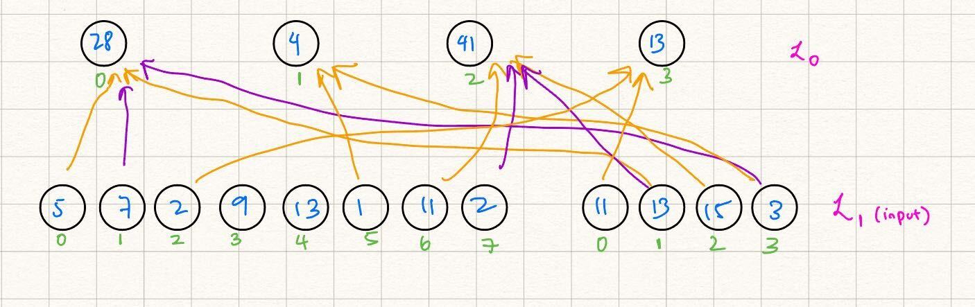
Code
The way we would represent the above diagram as a GKR circuit in Remainder is below, which can also be found in our codebase at frontend/examples/binary_gate.rs:
#![allow(unused)]
fn main() {
fn build_example_binary_gate_circuit<F: Field>(
    input_num_vars_lhs: usize,
    input_num_vars_rhs: usize,
    wiring: Vec<(u32, u32, u32)>,
    binary_operation: BinaryOperation,
    output_num_vars: usize,
) -> Circuit<F> {
    let mut builder = CircuitBuilder::<F>::new();

    let public = builder.add_input_layer("Public", LayerVisibility::Public);
    // The left-hand side candidates for the input to the binary gate
    let lhs_input = builder.add_input_shred("LHS candidates for binary gate", input_num_vars_lhs, &public);
    // The right-hand side candidates for the input to the binary gate
    let rhs_input = builder.add_input_shred("RHS candidates for binary gate", input_num_vars_rhs, &public);
    // The expected output of the gate operation
    let expected_output = builder.add_input_shred("Expected output", output_num_vars, &public);


    let gate_result = builder.add_gate_node(&lhs_input, &rhs_input, wiring, binary_operation, None);

    let output = builder.add_sector(gate_result - expected_output);
    builder.set_output(&output);

    builder.build().unwrap()
}

#[test]
pub fn binary_gate_example() {
    const LHS_NUM_VARS: usize = 3;
    const RHS_NUM_VARS: usize = 2;
    const OUTPUT_NUM_VARS: usize = 2;

    // Example inputs to the gate function
    let lhs_mle: MultilinearExtension<Fr> = vec![5, 7, 2, 9, 13, 1, 11, 2].into();
    let rhs_mle: MultilinearExtension<Fr> = vec![11, 13, 15, 3].into();
    // Example wiring
    let wiring = vec![
        (0, 0, 1),
        (0, 1, 3),
        (1, 5, 3),
        (2, 6, 2),
        (2, 7, 1),
        (3, 2, 0),
    ];
    let expected_output_mle: MultilinearExtension<Fr> = vec![28, 4, 41, 13].into();


    // Create circuit description
    let mut prover_circuit =
        build_example_binary_gate_circuit::<Fr>(LHS_NUM_VARS, RHS_NUM_VARS, wiring, BinaryOperation::Add, OUTPUT_NUM_VARS);
    let mut verifier_circuit = prover_circuit.clone();

    prover_circuit.set_input("LHS candidates for binary gate", lhs_mle.clone());
    prover_circuit.set_input("RHS candidates for binary gate", rhs_mle.clone());
    prover_circuit.set_input("Expected output", expected_output_mle.clone());

    let provable_circuit = prover_circuit.finalize().unwrap();

    // Prove the circuit
    let (proof_config, proof_as_transcript) =
        prove_circuit_with_runtime_optimized_config::<Fr, PoseidonSponge<Fr>>(&provable_circuit);

    // Create verifier circuit description and attach inputs.
    verifier_circuit.set_input("LHS candidates for binary gate", lhs_mle);
    verifier_circuit.set_input("RHS candidates for binary gate", rhs_mle);
    verifier_circuit.set_input("Expected output", expected_output_mle);

    let (verifiable_circuit, predetermined_public_inputs) =
        verifier_circuit.gen_verifiable_circuit().unwrap();
    verify_circuit_with_proof_config(
        &verifiable_circuit,
        predetermined_public_inputs,
        &proof_config,
        proof_as_transcript,
    );
}
}
Example 2: Identity Gate
Diagram
Let us define the following layerwise relationship, as a small GKR circuit:
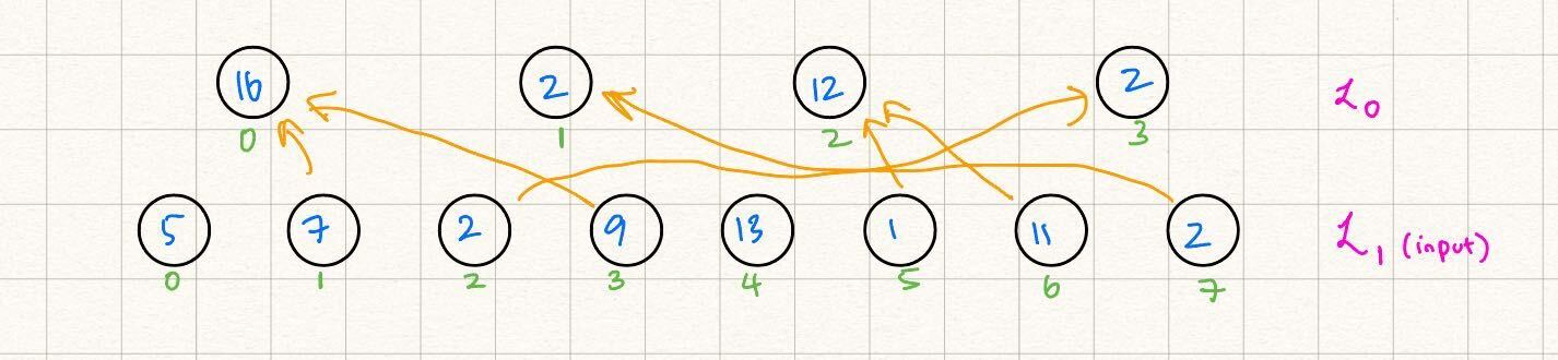
Code
The way we would represent the above diagram as a GKR circuit in Remainder is below, which can also be found in our codebase at frontend/examples/identity_gate.rs:
#![allow(unused)]
fn main() {
fn build_example_identity_gate_circuit<F: Field>(
    source_num_vars: usize,
    wiring: Vec<(u32, u32)>,
    output_num_vars: usize,
) -> Circuit<F> {
    let mut builder = CircuitBuilder::<F>::new();

    let public = builder.add_input_layer("Public", LayerVisibility::Public);
    // The MLE that we are routing via the wiring
    let source = builder.add_input_shred("Source for identity gate", source_num_vars, &public);
    // Expected result of the wiring
    let expected_output = builder.add_input_shred("Expected output", output_num_vars, &public);

    let gate_result = builder.add_identity_gate_node(&source, wiring, output_num_vars, None);

    let output = builder.add_sector(gate_result - expected_output);
    builder.set_output(&output);

    builder.build().unwrap()
}

#[test]
pub fn id_gate_example() {
    const SOURCE_NUM_VARS: usize = 3;
    const OUTPUT_NUM_VARS: usize = 2;

    // The example input MLE.
    let source_mle: MultilinearExtension<Fr> = vec![5, 7, 2, 9, 13, 1, 11, 2].into();
    // Example wiring.
    let wiring = vec![
        (0, 1),
        (0, 3),
        (1, 7),
        (2, 6),
        (2, 5),
        (3, 2),
    ];
    let expected_output_mle: MultilinearExtension<Fr> = vec![16, 2, 12, 2].into();


    // Create circuit description.
    let mut prover_circuit =
        build_example_identity_gate_circuit::<Fr>(SOURCE_NUM_VARS, wiring, OUTPUT_NUM_VARS);
    let mut verifier_circuit = prover_circuit.clone();

    prover_circuit.set_input("Source for identity gate", source_mle.clone());
    prover_circuit.set_input("Expected output", expected_output_mle.clone());

    let provable_circuit = prover_circuit.finalize().unwrap();

    // Prove the circuit.
    let (proof_config, proof_as_transcript) =
        prove_circuit_with_runtime_optimized_config::<Fr, PoseidonSponge<Fr>>(&provable_circuit);

    // Create verifier circuit description and attach inputs.
    verifier_circuit.set_input("Source for identity gate", source_mle);
    verifier_circuit.set_input("Expected output", expected_output_mle);

    let (verifiable_circuit, predetermined_public_inputs) =
        verifier_circuit.gen_verifiable_circuit().unwrap();
    verify_circuit_with_proof_config(
        &verifiable_circuit,
        predetermined_public_inputs,
        &proof_config,
        proof_as_transcript,
    );
}
}
Example 3: Dataparallel Binary Gate
Diagram
Let us define the following layerwise relationship, as a small GKR circuit:
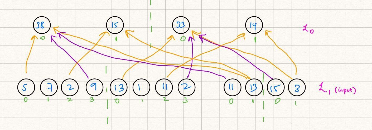
Code
The way we would represent the above diagram as a GKR circuit in Remainder is below, which can also be found in our codebase at frontend/examples/binary_gate_dataparallel.rs:
#![allow(unused)]

fn main() {
fn build_example_binary_gate_circuit_dataparallel<F: Field>(
    num_dataparallel_vars: usize,
    input_num_vars_lhs: usize,
    input_num_vars_rhs: usize,
    wiring: Vec<(u32, u32, u32)>,
    binary_operation: BinaryOperation,
    output_num_vars: usize,
) -> Circuit<F> {
    let mut builder = CircuitBuilder::<F>::new();

    let public = builder.add_input_layer("Public", LayerVisibility::Public);
    // The input candidates for the left-hand side of the gate
    let lhs_input = builder.add_input_shred("LHS candidates for binary gate", input_num_vars_lhs, &public);
    // The input candidates for the right-hand side of the gate
    let rhs_input = builder.add_input_shred("RHS candidates for binary gate", input_num_vars_rhs, &public);
    // The expected output of the gate operation
    let expected_output = builder.add_input_shred("Expected output", output_num_vars, &public);


    let gate_result = builder.add_gate_node(&lhs_input, &rhs_input, wiring, binary_operation, Some(num_dataparallel_vars));

    let output = builder.add_sector(gate_result - expected_output);
    builder.set_output(&output);

    builder.build().unwrap()
}

#[test]
pub fn binary_gate_dataparallel_example() {
    const NUM_DATAPARALLEL_VARS: usize = 1;
    const LHS_NUM_VARS: usize = 3;
    const RHS_NUM_VARS: usize = 2;
    const OUTPUT_NUM_VARS: usize = 2;

    // Example inputs
    let lhs_mle: MultilinearExtension<Fr> = vec![5, 7, 2, 9, 13, 1, 11, 2].into();
    let rhs_mle: MultilinearExtension<Fr> = vec![11, 13, 15, 3].into();
    // Example wiring: Is repeated across (1 << [NUM_DATAPARALLEL_VARS]) copies of the circuit
    let wiring = vec![
        (0, 0, 1),
        (0, 3, 0),
        (1, 2, 1),
    ];
    let expected_output_mle: MultilinearExtension<Fr> = vec![38, 15, 33, 14].into();


    // Create circuit description
    let mut prover_circuit =
        build_example_binary_gate_circuit_dataparallel::<Fr>(NUM_DATAPARALLEL_VARS, LHS_NUM_VARS, RHS_NUM_VARS, wiring, BinaryOperation::Add, OUTPUT_NUM_VARS);
    let mut verifier_circuit = prover_circuit.clone();

    prover_circuit.set_input("LHS candidates for binary gate", lhs_mle.clone());
    prover_circuit.set_input("RHS candidates for binary gate", rhs_mle.clone());
    prover_circuit.set_input("Expected output", expected_output_mle.clone());

    let provable_circuit = prover_circuit.finalize().unwrap();

    // Prove the circuit
    let (proof_config, proof_as_transcript) =
        prove_circuit_with_runtime_optimized_config::<Fr, PoseidonSponge<Fr>>(&provable_circuit);

    // Create verifier circuit description and attach inputs.
    verifier_circuit.set_input("LHS candidates for binary gate", lhs_mle);
    verifier_circuit.set_input("RHS candidates for binary gate", rhs_mle);
    verifier_circuit.set_input("Expected output", expected_output_mle);

    let (verifiable_circuit, predetermined_public_inputs) =
        verifier_circuit.gen_verifiable_circuit().unwrap();
    verify_circuit_with_proof_config(
        &verifiable_circuit,
        predetermined_public_inputs,
        &proof_config,
        proof_as_transcript,
    );
}

}
Example 4: Dataparallel Identity Gate
Diagram
Let us define the following layerwise relationship, as a small GKR circuit:
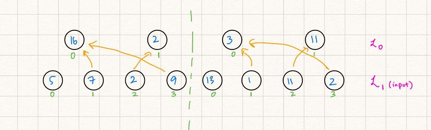
Code
The way we would represent the above diagram as a GKR circuit in Remainder is below, which can also be found in our codebase at frontend/examples/identity_gate_dataparallel.rs:
#![allow(unused)]
fn main() {
fn build_example_identity_gate_circuit_dataparallel<F: Field>(
    num_dataparallel_vars: usize,
    source_num_vars: usize,
    wiring: Vec<(u32, u32)>,
    output_num_vars: usize,
) -> Circuit<F> {
    let mut builder = CircuitBuilder::<F>::new();

    let public = builder.add_input_layer("Public", LayerVisibility::Public);
    // The MLE that we are routing via the wiring
    let source = builder.add_input_shred("Source for identity gate", source_num_vars, &public);
    // Expected routing result from the wiring
    let expected_output = builder.add_input_shred("Expected output", output_num_vars, &public);

    let gate_result = builder.add_identity_gate_node(&source, wiring, output_num_vars, Some(num_dataparallel_vars));

    let output = builder.add_sector(gate_result - expected_output);
    builder.set_output(&output);

    builder.build().unwrap()
}

#[test]
pub fn id_gate_dataparallel_example() {
    const NUM_DATAPARALLEL_VARS: usize = 1;
    const SOURCE_NUM_VARS: usize = 3;
    const OUTPUT_NUM_VARS: usize = 2;

    // Example input
    let source_mle: MultilinearExtension<Fr> = vec![5, 7, 2, 9, 13, 1, 11, 2].into();
    // Example wiring. This is repeated across (1 << [NUM_DATAPARALLEL_VARS]) copies of the circuit.
    let wiring = vec![
        (0, 1),
        (0, 3),
        (1, 2),
    ];
    let expected_output_mle: MultilinearExtension<Fr> = vec![16, 2, 3, 11].into();


    // Create circuit description
    let mut prover_circuit =
        build_example_identity_gate_circuit_dataparallel::<Fr>(NUM_DATAPARALLEL_VARS, SOURCE_NUM_VARS, wiring, OUTPUT_NUM_VARS);
    let mut verifier_circuit = prover_circuit.clone();

    prover_circuit.set_input("Source for identity gate", source_mle.clone());
    prover_circuit.set_input("Expected output", expected_output_mle.clone());

    let provable_circuit = prover_circuit.finalize().unwrap();

    // Prove the circuit
    let (proof_config, proof_as_transcript) =
        prove_circuit_with_runtime_optimized_config::<Fr, PoseidonSponge<Fr>>(&provable_circuit);

    // Create verifier circuit description and attach inputs.
    verifier_circuit.set_input("Source for identity gate", source_mle);
    verifier_circuit.set_input("Expected output", expected_output_mle);

    let (verifiable_circuit, predetermined_public_inputs) =
        verifier_circuit.gen_verifiable_circuit().unwrap();
    verify_circuit_with_proof_config(
        &verifiable_circuit,
        predetermined_public_inputs,
        &proof_config,
        proof_as_transcript,
    );
}
}
MatMult Layer Usage Tutorial
Let's see how we can use a MatMult layer to prove the computation of the following matrix
product:
Recall that a MatMult layer requires all dimensions of all the
matrices involved in the product to be exact powers of two. We can always guarantee this
property by padding the original matrices with zero columns and/or rows as follows:
How do we represent matrices as MLEs? In Remainder's implementation of the MatMult layer, we
follow the convention of representing an matrix as an MLE whose evaluations on the
hypercube are given by a vector in
which represents a row-major flattened view of the matrix.
For example, here's how we'd represent matrices defined above as MLEs:
A MatMult layer is a specialized layer which, given the MLEs
representing matrices , it
computes the output MLE representing matric such
that .
To prove the computation of matrix product in Remainder, we can simply subtract the expected
from the result of the MatMult layer and constraine the result to be the all-zero
vector.
The only remaining complication to address is that typically it's not reasonable to expect the input to be given in an already padded form. In such a case, we'd have to perform the padding in circuit. In the example above, this would mean transforming MLE representations of matrices , to the MLEs .
This is easy to do with an Identity Gate layer, as we'll see in the following example.
Example: Input given in un-padded row-major order
A natural way to represent the original, unpadded matrices given previously, would be by just flattening the matrices in row-major order, as the following MLEs:
Notice how in this case the MLEs for matrices are already in the expected format. And in fact this will be the case every time the number of columns is an exact power of two. The number of rows doesn't really affect the matrix padding because Remainder is already implicitly padding every MLE with zeros when the number of evaluations given is not an exact power of two.
Notice however that this implicit padding is not the same as the matrix padding we described
earlier. Compare for example the MLE given earlier, with that of
. To pad matrix in the way MatMult expects, we can use custom
wirings on an Identity Gate Layer to re-wire the values of MLE into
the right places and get MLE . In this case the wiring look like:

Here's the complete code for this example, which can also be found in our repository
atfrontend/examples/matmult.rs:
#![allow(unused)]
fn main() {
const PADDED_MATRIX_A_LOG_NUM_ROWS: usize = 2;
const PADDED_MATRIX_A_LOG_NUM_COLS: usize = 2;
const PADDED_MATRIX_B_LOG_NUM_ROWS: usize = 2;
const PADDED_MATRIX_B_LOG_NUM_COLS: usize = 1;

const MATRIX_A_NUM_VARS: usize = 4;
const MATRIX_B_NUM_VARS: usize = 3;
const MATRIX_C_NUM_VARS: usize = 3;

let matrix_a_data: MultilinearExtension<Fr> = vec![0, 1, 2, 1, 2, 3, 2, 3, 4].into();
let matrix_b_data: MultilinearExtension<Fr> = vec![3, 4, 4, 5, 5, 6].into();
let matrix_c_data: MultilinearExtension<Fr> = vec![14, 17, 26, 32, 38, 47].into();

let matrix_a_padding_wiring = vec![
    (0, 0),
    (1, 1),
    (2, 2),
    (4, 3),
    (5, 4),
    (6, 5),
    (8, 6),
    (9, 7),
    (10, 8),
];

let mut builder = CircuitBuilder::<Fr>::new();

let inputs = builder.add_input_layer("Matrices", LayerVisibility::Public);

let matrix_a = builder.add_input_shred("Matrix A", MATRIX_A_NUM_VARS, &inputs);
let matrix_b = builder.add_input_shred("Matrix B", MATRIX_B_NUM_VARS, &inputs);
let expected_matrix_c =
    builder.add_input_shred("Expected Matrix C", MATRIX_C_NUM_VARS, &inputs);

let padded_matrix_a =
    builder.add_identity_gate_node(&matrix_a, matrix_a_padding_wiring, MATRIX_A_NUM_VARS, None);

let matrix_c = builder.add_matmult_node(
    &padded_matrix_a,
    (PADDED_MATRIX_A_LOG_NUM_ROWS, PADDED_MATRIX_A_LOG_NUM_COLS),
    &matrix_b,
    (PADDED_MATRIX_B_LOG_NUM_ROWS, PADDED_MATRIX_B_LOG_NUM_COLS),
);

let output = builder.add_sector(matrix_c - expected_matrix_c);
builder.set_output(&output);

let circuit = builder.build().unwrap();

// Create circuit description.
let mut prover_circuit = circuit.clone();
let mut verifier_circuit = circuit.clone();

prover_circuit.set_input("Matrix A", matrix_a_data.clone());
prover_circuit.set_input("Matrix B", matrix_b_data.clone());
prover_circuit.set_input("Expected Matrix C", matrix_c_data.clone());

let provable_circuit = prover_circuit.gen_provable_circuit().unwrap();

// Prove the circuit.
let (proof_config, proof_as_transcript) =
    prove_circuit_with_runtime_optimized_config::<Fr, PoseidonSponge<Fr>>(&provable_circuit);

// Create verifier circuit description and attach inputs.
verifier_circuit.set_input("Matrix A", matrix_a_data);
verifier_circuit.set_input("Matrix B", matrix_b_data);
verifier_circuit.set_input("Expected Matrix C", matrix_c_data);

let verifiable_circuit = verifier_circuit.gen_verifiable_circuit().unwrap();
verify_circuit_with_proof_config(&verifiable_circuit, &proof_config, proof_as_transcript);
}
Note: In the previous example we hard-coded the wirings corresponding to the case of padding a * matrix MLE. For the general case, one can easily generate the correct wirings for *padding for any matrix dimensions.
Example 1: u8 range check
The following example, building on the section where we discuss LogUp Theory, uses a lookup to check that the provided values are in the range .
See also frontend/examples/lookup.rs:
fn build_example_lookup_circuit<F: Field>(
    table_num_vars: usize,
    witness_num_vars: usize,
) -> Circuit<F> {
    let mut builder = CircuitBuilder::<F>::new();

    // Lookup table is typically public
    let public = builder.add_input_layer("Public", LayerVisibility::Public);
    let table = builder.add_input_shred("Table", table_num_vars, &public);

    // Witness values are typically private, as are multiplicities
    let private = builder.add_input_layer("Private", LayerVisibility::Private);
    let witness = builder.add_input_shred(
        "Witness",
        witness_num_vars,
        &private,
    );
    let multiplicities = builder.add_input_shred(
        "Multiplicities",
        table_num_vars,
        &private,
    );

    // Create the circuit components
    let fiat_shamir_challenge_node = builder.add_fiat_shamir_challenge_node(1);
    let lookup_table = builder.add_lookup_table(&table, &fiat_shamir_challenge_node);
    let _lookup_constraint = builder.add_lookup_constraint(
        &lookup_table, &witness, &multiplicities);

    builder.build().unwrap()
}

/// Example demonstrating a range check using a lookup table.
fn main() {
    const TABLE_NUM_VARS: usize = 8;
    const WITNESS_NUM_VARS: usize = 2;
    const RANGE_LIMIT: u64 = 1 << TABLE_NUM_VARS; // 256

    // The lookup table contains the values 0 thru 255
    let table_mle = MultilinearExtension::new(
        (0u64..RANGE_LIMIT).map(|x| Fr::from(x)).collect(),
    );
    // Some example witness values to be range checked
    let witness_values = vec![233u64, 233u64, 0u64, 1u64];
    // Count the number of times each value occurs to build the multiplicities MLE.
    let mut multiplicities: Vec<u32> = vec![0; RANGE_LIMIT as usize];
    witness_values.iter().for_each(|value| {
            multiplicities[*value as usize] += 1;
    });
    let witness_mle: MultilinearExtension<Fr> = witness_values.into();
    let multiplicities_mle: MultilinearExtension<Fr> = multiplicities.into();

    // Create circuit description
    let mut prover_circuit =
        build_example_lookup_circuit::<Fr>(TABLE_NUM_VARS, WITNESS_NUM_VARS);
    let mut verifier_circuit = prover_circuit.clone();

    prover_circuit.set_input("Table", table_mle.clone());
    prover_circuit.set_input("Witness", witness_mle);
    prover_circuit.set_input("Multiplicities", multiplicities_mle);

    let provable_circuit = prover_circuit.finalize().unwrap();

    // Prove the circuit
    let (proof_config, proof_as_transcript) =
        prove_circuit_with_runtime_optimized_config::<Fr, PoseidonSponge<Fr>>(&provable_circuit);

    // Create verifier circuit description and attach lookup table as public
    // input to it.
    verifier_circuit.set_input("Table", table_mle);
    let (verifiable_circuit, predetermined_public_inputs) =
        verifier_circuit.gen_verifiable_circuit().unwrap();
    verify_circuit_with_proof_config(
        &verifiable_circuit,
        predetermined_public_inputs,
        &proof_config,
        proof_as_transcript,
    );
}
Example 2: sigmoid function
The following example uses an indexed lookup to check that the provided input and output values correspond under the sigmoid function.
Inputs and outputs are both scaled and discretized: for all integers , the corresponding field element represents the real value .
See also remainder_frontend/examples/indexed_lookup.rs:
fn build_example_indexed_lookup_circuit<F: Field>(
    table_num_vars: usize,
    witness_num_vars: usize,
) -> Circuit<F> {
    let mut builder = CircuitBuilder::<F>::new();

    // Lookup table is typically public
    let public = builder.add_input_layer("Public", LayerVisibility::Public);
    let table_input = builder.add_input_shred("Table input", table_num_vars, &public);
    let table_output = builder.add_input_shred("Table output", table_num_vars, &public);

    // Witness values are typically private, as are multiplicities
    let private = builder.add_input_layer("Private", LayerVisibility::Private);
    let witness_input = builder.add_input_shred(
        "Witness input",
        witness_num_vars,
        &private,
    );
    let witness_output = builder.add_input_shred(
        "Witness output",
        witness_num_vars,
        &private,
    );
    let multiplicities = builder.add_input_shred(
        "Multiplicities",
        table_num_vars,
        &private,
    );

    // A Fiat-Shamir challenge node is needed to combine input and output values
    let rlc_fiat_shamir_challenge_node = builder.add_fiat_shamir_challenge_node(1);

    // Combine input and output values for the indexed lookup
    let table_values = builder.add_sector(&table_input + &rlc_fiat_shamir_challenge_node * &table_output);
    let witness_values = builder.add_sector(&witness_input + &rlc_fiat_shamir_challenge_node * &witness_output);

    // Add the usual lookup components
    let logup_fiat_shamir_challenge_node = builder.add_fiat_shamir_challenge_node(1);
    let lookup_table = builder.add_lookup_table(&table_values, &logup_fiat_shamir_challenge_node);
    let _lookup_constraint = builder.add_lookup_constraint(
        &lookup_table, &witness_values, &multiplicities);

    builder.build().unwrap()
}

fn main() {
    // Uses an indexed lookup to check the application of a function defined by a lookup table.
    // The sigmoid function is used.
    // Inputs and outputs are both scaled and discretized: for all integers `2^9 <= i < 2^9`, the corresponding field element $i \in \mathbb{F}$ represents the real value $i / 2^8$.
    const TABLE_NUM_VARS: usize = 10;
    const WITNESS_NUM_VARS: usize = 2;
    let range_limit: i64 = 1 << (TABLE_NUM_VARS - 1);

    let sigmoid = |x: i64| -> i64 {
        // Sigmoid function scaled by 2^5
        let x_real = (x as f64) / 32.0;
        let sigmoid_real = 1.0 / (1.0 + (-x_real).exp());
        (sigmoid_real * 32.0).round() as i64
    };

    // The lookup table will contain the input and output values for the sigmoid for input values
    let input_values_mle: MultilinearExtension<Fr> = (-range_limit..range_limit).collect::<Vec<_>>().into();
    let output_values_mle: MultilinearExtension<Fr> = (-range_limit..range_limit)
        .map(|x| sigmoid(x))
        .collect::<Vec<_>>()
        .into();

    // Some example witness input values to be evaluated through the lookup table
    let witness_input_values = vec![-20i64, 0i64, 12i64, 12i64];
    let witness_output_values: Vec<i64> = witness_input_values
        .iter()
        .map(|&x| sigmoid(x))
        .collect();
    let witness_input_mle: MultilinearExtension<Fr> = witness_input_values.clone().into();
    let witness_output_mle: MultilinearExtension<Fr> = witness_output_values.into();

    // Count the number of times each (input, output) pair occurs to build the multiplicities MLE.
    let mut multiplicities : Vec<u32> = vec![0; 1 << TABLE_NUM_VARS];
    witness_input_values.iter().for_each(|&input_value| {
        // Compute the index in the table for the (input, output) pair
        let index = input_value + range_limit;
        multiplicities[index as usize] += 1;
    });
    let multiplicities_mle: MultilinearExtension<Fr> = multiplicities.into();

    // Create circuit description
    let mut prover_circuit =
        build_example_indexed_lookup_circuit::<Fr>(TABLE_NUM_VARS, WITNESS_NUM_VARS);
    let mut verifier_circuit = prover_circuit.clone();

    prover_circuit.set_input("Table input", input_values_mle.clone());
    prover_circuit.set_input("Table output", output_values_mle.clone());
    prover_circuit.set_input("Witness input", witness_input_mle.clone());
    prover_circuit.set_input("Witness output", witness_output_mle.clone());
    prover_circuit.set_input("Multiplicities", multiplicities_mle);

    let provable_circuit = prover_circuit.finalize().unwrap();

    // Prove the circuit
    let (proof_config, proof_as_transcript) =
        prove_circuit_with_runtime_optimized_config::<Fr, PoseidonSponge<Fr>>(&provable_circuit);

    // Create verifier circuit description and attach lookup table as public
    // input to it.
    verifier_circuit.set_input("Table input", input_values_mle);
    verifier_circuit.set_input("Table output", output_values_mle);
    let (verifiable_circuit, predetermined_public_inputs) =
        verifier_circuit.gen_verifiable_circuit().unwrap();
    verify_circuit_with_proof_config(
        &verifiable_circuit,
        predetermined_public_inputs,
        &proof_config,
        proof_as_transcript,
    );
}
Hyrax Frontend Tutorial
This tutorial closely resembles the one for Remainder's GKR prover/verifier,
i.e. the one written in the quickstart section. The code
for the Hyrax frontend tutorial is here, and can be run from the Remainder_CE
root directory via the following command:
cargo run --package frontend --example hyrax_tutorial
Note that although this tutorial is a code-only, standalone tutorial, we would very strongly encourage you to read through at least the Hyrax introduction section to get a better understanding of what the various code pieces represent and why Hyrax is one of several options for converting GKR into a fully zero-knowledge protocol.
Setting up the circuit
This uses the exact same code/circuit as the one from the quickstart,
and we encourage you to check out that section to understand the structure of
the circuit described here. Indeed, the Circuit<F> generation function within
frontend/examples/hyrax_tutorial.rs is a copy/paste of the one in frontend/examples/tutorial.rs.
As a quick reminder, the circuit we defined (see build_circuit()) has two
input layers, one private/committed and one public. The private/committed input
layer contains two sub-inputs, "LHS" and "RHS", and the public input layer contains
a single sub-input, "Expected output". In the GKR case/tutorial, we used the (non-ZK)
Ligero PCS to commit to and open the committed
input layer at a challenge point, and in the Hyrax case, the prover will be
using the zero-knowledge Hyrax PCS to do the same.
#![allow(unused)]
fn main() {
let lhs_rhs_input_layer =
    builder.add_input_layer("LHS RHS input layer", LayerVisibility::Committed);
let expected_output_input_layer =
    builder.add_input_layer("Expected output", LayerVisibility::Public);
}
Recall that we create two copies of the Circuit<F>: one for the prover (to
attach private and public input data to), and one for the verifier (no data
attached):
#![allow(unused)]
fn main() {
// Create the base layered circuit description.
let base_circuit = build_circuit();
let mut prover_circuit = base_circuit.clone();
let verifier_circuit = base_circuit.clone();
}
Similarly to the GKR tutorial, we generate input data for the circuit and attach them to the prover circuit:
#![allow(unused)]
fn main() {
// Generate circuit inputs.
let lhs_data = vec![1, 2, 3, 4].into();
let rhs_data = vec![5, 6, 7, 8].into();
let expected_output_data = vec![5, 12, 21, 32].into();

// Append circuit inputs to their respective input "shreds" in the prover's
// view of the circuit.
prover_circuit.set_input("LHS", lhs_data); // This is committed!
prover_circuit.set_input("RHS", rhs_data); // This is committed!
prover_circuit.set_input("Expected output", expected_output_data); // This is public!
}
Setting up the proving environment
Next, we create a pair of proving/verification configs. We won't elaborate on the specific configuration options here, but the idea is that they are effectively a group of global context variables which affect certain proving/verification options (e.g. trading off runtime vs. memory usage, whether to use certain optimizations, etc.). Note that in the quickstart, we hid the config + macro API with another wrapper for simplicity, but are exposing the options here. For now, we will stick with the "Hyrax compatible runtime-optimized default" option:
#![allow(unused)]
fn main() {
// Create GKR circuit prover + verifier configs which work with Hyrax
let hyrax_circuit_prover_config =
    GKRCircuitProverConfig::hyrax_compatible_runtime_optimized_default();
let hyrax_circuit_verifier_config =
    GKRCircuitVerifierConfig::new_from_prover_config(&hyrax_circuit_prover_config, false);
}
Similarly to how we needed to create a ProvableCircuit<F> in the GKR tutorial,
we invoke a similar function here, gen_hyrax_provable_circuit(), to gather our
previously attached circuit inputs and prepare the circuit for proving:
#![allow(unused)]
fn main() {
// Create a version of the circuit description which the prover can use.
// Note that in this case, we create a "Hyrax-provable" circuit rather than
// a "GKR-provable" one.
let mut hyrax_provable_circuit: HyraxProvableCircuit<Bn256Point> = prover_circuit
    .gen_hyrax_provable_circuit()
    .expect("Failed to generate provable circuit");
}
Next, we prepare a couple of structs which are specific to Hyrax proving. First, we create a Pedersen committer, which creates and keeps track of the group generators to be used in proving (see our Hyrax overview and Pedersen commitments sections for more details here).
Importantly, the public string used to instantiate the committer must be agreed upon between the prover and verifier. This ensures a "nothing-up-my-sleeve number" verification setting where a malicious prover cannot cheat by picking a set of generators for which they e.g. know a discrete log relationship between, which would allow them to break the soundness of the protocol:
#![allow(unused)]
fn main() {
// The Pedersen committer creates and keeps track of the shared generators
// between the prover and verifier. Note that the generators are created
// deterministically from the public string.
let prover_pedersen_committer =
    PedersenCommitter::new(512, "Hyrax tutorial Pedersen committer", None);
}
Next, we set up the RNG required for generating blinding factors within the protocol -- note that the example used here is insecure for simplicity. In practice, please instantiate the blinding factor RNG with a CSPRNG.
#![allow(unused)]
fn main() {
// WARNING: This is for tutorial purposes ONLY. NEVER use anything but a CSPRNG for generating blinding factors!
let mut blinding_rng = thread_rng();
}
Finally, we set up an inverse Vandermonde matrix, which helps us convert univariate polynomials from evaluation to coefficient form. This is helpful for the Hyrax verifier in the interpolative claim aggregation case, since can only be easily evaluated by the verifier when the polynomial is sent in Pedersen commitments to coefficients rather than evaluations:
#![allow(unused)]
fn main() {
// The Vandermonde inverse matrix allows us to convert from evaluations
// to coefficients for interpolative claim aggregation. Note that the
// coefficient form allows the verifier to directly check relationships
// via the homomorphic properties of the curve.
let mut vandermonde_converter = VandermondeInverse::new();
}
Proving
We instantiate a prover transcript over the protocol's elliptic curve's base field for Fiat-Shamir:
#![allow(unused)]
fn main() {
// Finally, we instantiate a transcript over the base field. Note that
// prover messages are elliptic curve points which can be encoded as base
// field tuples, while verifier messages are scalar field elements of that
// curve. Thanks to Hasse's theorem, this results in a negligible completeness
// loss in the non-interactive case as we always attempt to coerce a base
// field challenge into a scalar field element and panic if the base field
// element sampled was larger than the scalar field modulus.
let mut prover_transcript: ECTranscript<Bn256Point, PoseidonSponge<Fq>> =
    ECTranscript::new("Hyrax tutorial prover transcript");
}
We are finally ready to generate the Hyrax proof! Note that the
perform_function_under_prover_config!() macro ensures (even within a
multi-threaded environment) that the function passed in will only be called
and be run in its entirety under the state set by hyrax_circuit_prover_config.
#![allow(unused)]
fn main() {
// Use the `perform_function_under_prover_config!` macro to run the
// Hyrax prover's `prove` function with the above arguments, under the
// prover config passed in.
let (proof, proof_config) = perform_function_under_prover_config!(
    // This is a hack to get around the macro's syntax for struct methods
    // rather than function calls.
    |w, x, y, z| hyrax_provable_circuit.prove(w, x, y, z),
    &hyrax_circuit_prover_config,
    &prover_pedersen_committer,
    &mut blinding_rng,
    &mut vandermonde_converter,
    &mut prover_transcript
);
}
Verification
Similarly to the verification process in the GKR tutorial, we first collect verifier-known inputs (in this case, there are none) and create a (Hyrax) verifier-ready version of the circuit:
#![allow(unused)]
fn main() {
// We generate a "Hyrax-verifiable" circuit from the `Circuit` struct,
// but do not attach any circuit inputs to it (these must come from
// the proof itself).
let hyrax_verifiable_circuit = verifier_circuit
    .gen_hyrax_verifiable_circuit()
    .expect("Failed to generate Hyrax verifiable circuit");
}
The verifier creates its own Pedersen committer and derives the agreed-upon generators from scratch:
#![allow(unused)]
fn main() {
// The verifier can (and should) derive the elliptic curve generators on
// its own from the public string and check the proof against these.
let verifier_pedersen_committer =
    PedersenCommitter::new(512, "Hyrax tutorial Pedersen committer", None);
}
Finally, the verifier instantiates its own Fiat-Shamir transcript:
#![allow(unused)]
fn main() {
// The verifier instantiates its own transcript.
let mut verifier_transcript: ECTranscript<Bn256Point, PoseidonSponge<Fq>> =
    ECTranscript::new("Hyrax tutorial verifier transcript");
}
And we commence verification using the perform_function_under_verifier_config!()
macro, which is identical in behavior to the above perform_function_under_prover_config!()
macro call, but with consistency against the hyrax_circuit_verifier_config
rather than the prover one.
#![allow(unused)]
fn main() {
// Finally, we verify the proof using the above committer + transcript, as
// well as the Hyrax verifier config generated from the prover one earlier.
perform_function_under_verifier_config!(
    verify_hyrax_proof,
    &hyrax_circuit_verifier_config,
    &proof,
    &hyrax_verifiable_circuit,
    &verifier_pedersen_committer,
    &mut verifier_transcript,
    &proof_config
);
}
And that's it! You've now created your first Hyrax-provable/verifiable circuit and generated and verified a Hyrax zero-knowledge proof. Note that aside from the couple of additional structs we needed to supply to the prover/verifier (e.g. the Pedersen committer, the blinding factor RNG, the Vandermonde inverse matrix, and defining the curve whose scalar field is the one used in the circuit), the entire circuit definition + input data attachment process was identical to that of the GKR tutorial from earlier -- this is all by design, and in large part due to the fact that so many of the GKR prover/verifier operations can be so neatly wrapped (if done carefully and modular-ly) by Pedersen commitments!
Hyrax Interactive Protocol
Hyrax is a transformation to the GKR protocol which makes it zero knowledge. The GKR protocol as explained in our GKR Tutorial is not zero knowledge on its own. Recall that in the section about what GKR Proofs look like, we mention that GKR proofs contain the sumcheck messages from the sumcheck protocol performed for each layer of the arithmetic circuit.
Each of these sumcheck messages are the evaluations of a very particular univariate polynomial, constructed based on the data contained within that layer. Therefore, each of these evaluations leak a little bit of information on the data contained within a circuit, and these can be used to construct a system of equations that reveal some information about private inputs to a circuit.
Therefore, in use cases which require a zero knowledge proof of the output of a circuit, we use the Hyrax interactive protocol to transform GKR circuits into a variant which produces a zero knowledge proof. The high-level overview of the protocol is that rather than sending evaluations of the univariates directly, sends Pedersen commitments of these evaluations, and is able to verify these commitments to sumcheck messages by taking advantage of the additive homomorphism of Pedersen commitments.
For the remainder of this chapter we use additive group notation because this is the notation our code in Remainder is written in.
Background
The Hyrax protocol is defined over any cyclic group of prime order. We break down what this means below.
- Group: A group is an algebraic structure which is closed under a chosen binary operation, usually called the group operation. This means that if and , and the group operation of is denoted by , . Additionally, satisfies the following properties:
- Associativity: .
- Identity such that .
- Inverses such that .
- Order: The number of elements in a group, denoted by .
- Finite: is finite if it has finitely many elements.
- Cyclic: is cyclic if it contains a generator such that such that . In this case, we say that is generated by , meaning by composing with itself times, where and , we can enumerate every element of
- Prime Order: A group has prime order if is prime.
In Remainder, we instantiate Hyrax over an elliptic curve group, denoted below as , with prime order (defined by the trait PrimeOrderCurve).
Elliptic curve consists of points in a finite field satisfying the equation . An elliptic curve group's binary operation is "point addition," which we denote with . If we add to itself times, we call this operation "scalar multiplication," denoted by . While we won't go into full detail on elliptic curves in this tutorial, we define some operations that will make it easier to follow the rest of this section and the codebase. For more information on elliptic curves, you can read these notes on an introduction to elliptic curves.
-
Base Field: If , is defined by coordinates on a plane (either two or three, depending on the notation being used as explained below). Each of the coordinates of belong to the base field, which we denote as For example, if , then .
-
Scalar Field: The scalar field is the field , where , whose equivalence classes are the integers In other words, because is cyclic, it contains a generator , for some
-
Group Element: A group element is a point on the coordinate plane, and can be represented in many ways. We present the three types of representations used in the Remainder codebase below:
- Affine Coordinates: Affine coordinates are elliptic curve points represented in the traditional 2D plane, and are denoted as .
- Projective Coordinates: Projective coordinates are points on the projective plane, represented by where each point is the value in the appropriate dimension. To convert an affine coordinate to its projective coordinates, simply multiply each coordinate by some element to get . For every affine coordinate, there is a class of projective coordinates that define the same point. To go from a projective coordinate to its equivalent affine coordinate, the value is simply .
- Jacobian Coordinates: A jacobian coordinate represents the affine coordinate .
-
Point at Infinity: Note that it is not possible to define the appropriate affine coordinate corresponding to a projective coordinate if This is exactly the point at infinity, represented by the point .
Roadmap
For the rest of this chapter, we will first cover the Hyrax primitives, which allows us to prove properties of different blinded Pedersen commitments, such as proving that two commitments which look different (are different group elements) commit to the same message without having to open the commitment, or that the prover knows the message used to produce a commitment without having to open the commitment. We then move on to more complex proofs over Pedersen commitments such as Proof of Sumcheck and Proof of Claim Aggregation which prove that the prover has properly executed sumcheck or claim aggregation. Finally, we show how the primitives and more intermediate protocols can be put together to produce a valid GKR proof which only consists of blinded Pedersen commitments.
Pedersen Commitments
We continue to work in the elliptic curve group of prime order in this section with the group operation of point addition (denoted by ). Pedersen commitments are based on the discrete logarithm hardness assumption. Let be the generator of . This hardness assumption states that given a group element , and knowing , it is computationally hard to find the "discrete logarithm" of , namely, the scalar field element such that .
Commitment Schemes
Before explaining what Pedersen commitments are, we briefly provide background on commitment schemes. Commitment schemes allow a party to commit to a message in the form of a commitment . Note that the setup and definition for a polynomial commitment scheme is similar but with some subtle differences, as polynomial commitment schemes deal with committing to a message which is a bounded-degree polynomial such that a proof for evaluation at a later-determined point can be provided, while a commitment scheme in the sense of a Pedersen commitment more generally commits to a message (and can also be used as a PCS via proof-of-dot-product).
Properties
Commitment schemes are best described by the properties they satisfy. We informally define them below:
- Hiding: This gives privacy to the party computing the commitment. I.e., given a commitment , it is computationally difficult to extract the message it was computed from. A stronger notion, the "statistical hiding" property, says that the distribution of commitments that could be computed from a message is computationally indistinguishable from the distribution of commitments that could be computed from a message .
- Binding: This property gives security to the party receiving the commitment. It states that once given a commitment , the party who receives the commitment can be confident with up to negligible probability that the sender is tied to the message was computed from. In other words, the probability that is the commitment of two different messages is very low.
Protocol
Commitment schemes entail two phases:
- Commitment Phase: In the commitment phase, computes the commitment to its desired message and sends it to .
- Evaluation Phase: In the evaluation phase, receives the commitment and verifies (the actual method of verifying depends on which commitment scheme is being used) whether is indeed the commitment to the correct message .
Pedersen Commitment Construction
A Pedersen Commitment is one way of committing to a message, a construction used throughout the Hyrax interactive protocol. Pedersen commitments require a transparent set-up where both and agree on a generator .
Single Message Commitment
We commit to a message by simply computing . By the discrete log hardness assumption, it is hard to extract from , and because is a generator, can only be generated from .
Vector Pedersen Commitment
We commit to a list of messages by first agreeing on generators and then computing . This is what is normally referred to as a multi-scalar multiplication in elliptic-curve cryptography.
Blinded Pedersen Commitment
In Remainder, we use blinded Pedersen commitments in order to guarantee statistical zero-knowledge (produce statistically hiding commitments as explained above). This involves the prover holding a random tape (usually instantiated by a cryptographic pseudo-random number generator), and the prover and verifier agreeing beforehand on a "blinding generator" . The prover simply adds , which sampled from the random tape to its original, either Pedersen scalar commitment or vector commitment, to produce a blinded commitment. More succinctly, the blinded Pedersen commitment to a message is .
We go over how can verify that is indeed the commitment to a set of messages in future sections. Note that the size of both of these commitments is a single elliptic curve point, but the cost of computing these varies on the number of messages.
Hyrax Primitives
We go over various sigma protocols (interactive proofs with just 3 rounds of interaction) that allow the prover to prove various statements on its committed messages without having to open the commitment. For all of these protocols, let be the message commitment generators, and be the blinding generator. Let be the scalar field of . Assume the prover produces the blinding factor using a cryptographic PRNG.
Proof of Opening
In a Proof of Opening, shows that given a commitment , knows the message and blinding factor used to generate this commitment.
- samples uniformly from the scalar field. computes and sends over
- A random challenge from .
- , and .
- checks:
Proof of Equality
In a Proof of Equality, convinces that two commitments and commit to the same value, i.e. . In other words knows that , but only has the blinded commitments, which look uniformly random (since are uniformly randomly distributed in for uniformly random ).
- first uniformly samples a random value from . computes and sends to .
- A random challenge from .
- checks:
Proof of Product
Proof of product shows that a commitment is a commitment to the product of the messages committed to in and In other words, knows that and wants to prove this to without revealing the messages and just using the commitments.
- uniformly samples from and computes and sends over
- A random challenge from .
- checks:
Proof of Dot Product
Given 's commitment to a vector , and a public vector (known to both and ), and 's commitment to the claimed dot product , which is shows that they know a vector and blinding such that is equal to the message committed to in , and is a vector commitment for with blinding factor .
- samples a random vector in , . samples and computes and sends
- A random challenge from .
4. checks:
Proof of Sumcheck
A key observation that the Hyrax protocol makes is that the verifier's sumcheck "checks," i.e. that , and the final oracle query, can be modeled as linear equations.
At each round, "sends" the univariate by committing to its coefficients using Pedersen scalar commitments. Let (to get commitments ) be the coefficients for a degree univariate, where is the coefficient of the -th degree term.
Notice that is simply and is . Then is . We can compute the commitment to this using just the commitments to the coefficients as . Similarly, the evaluation can be computed using commitments to the coefficients of as . For each intermediate round of sumcheck, we simply have to compute a proof of equality between the two commitments and .
We can formulate the verifier's checks as a matrix vector product where the matrix contains the linear combination coefficients over the prover's messages, and the vector contains the prover's sumcheck messages as coefficients of the univariate polynomial in each round. Let round 's univariate have coefficients. Then, we can write the verifier's checks as such:
To encode all of the verifier's sumcheck checks in one go, we have check that:
The final represents the fact that the final dot product in the matrix-vector product is not . In fact, it should be exactly equal to the value that receives when it does the final "oracle query" in sumcheck. This is discussed next.
Every non-specified entry in the matrix is , and it has dimension . has dimension . Its product has dimension . The sum represents 's original claim for the sumcheck expression -- the sum of the first univariate should be equal to the sum, which is what the first row of the matrix multiplied by encodes.
Note that we can do a proof of dot product for each of the row of the matrix with as the private vector, and each entry in the resultant vector as the claimed dot product.
However, there is a small subtlety: every coefficients in must be committed to before the challenge is sampled for sumcheck. Otherwise, can modify the commitments to make false claims using its knowledge of Therefore, is committed to incrementally, and after each commitment is sampled. Finally, and engage in a proof of dot product for every row of the matrix .
The final "oracle query"
Over here we have encoded all of 's checks except for the final oracle query. Recall that at the end of sumcheck, has claims on underlying MLEs. In the Hyrax universe, commits to the claims it has on each of these MLEs, say via the commitments Then can combine these commitments linearly to compute a commitment to the expected value Then, we expand the matrix to have additional columns and add the coefficients needs to compute the linear combination of to the last (the -th) row of , and has additional entries with the commitments . Then can expect the result of the final dot product to be .
Example
We provide a minimal example to show how and are constructed. Assume and are engaging in sumcheck over the claim that , and via layerwise encoding, There are rounds of sumcheck (for each of the and ) variables, where bind to and is bound to . At the end of sumcheck, commits to and as and
look like this:
And their result that expects, which it can compute on its own is:
Optimizations
There is an optimization specified in the original Hyrax paper which allows us to take the random linear combination of the rows of and do proofs of dot product of just size where is the number of coefficients in the univariate of round , rather than proofs of dot product of size . We don't go into how to formulate this optimization, but suggest reading the original paper and specifically the "squashing 's checks" section. We have implemented this optimization in Remainder.
Proof of Claim Aggregation
There are two main methods of GKR claim aggregation used in Remainder, and we must provide proof that claims have been aggregated correctly for both methods, Random Linear Combination (RLC) and Interpolative Claim Aggregation, within the Hyrax framework as well.
Random Linear Combination (RLC) Claim Aggregation
Recall that RLC claim aggregation does not require a specific claim aggregation step, but rather just modifies the sumcheck equation for the next round. Therefore, the Hyrax does not need to provide a separate proof of claim aggregation, but instead in its proof of sumcheck, takes the random linear combination of the or polynomials when computing the expected value of the "oracle query."
Interpolative Claim Aggregation
For interpolative claim aggregation, however, aggregates a set of claims given a challenge from , and and engage in sumcheck over this single claim. When working in the Hyrax proof system, must prove, via Pedersen commitments, that it computed the correct aggregated claim. In interpolative claim aggregation, computes and sends a polynomial (defined in the GKR interpolative claim aggregation section referenced earlier). Instead of sending this polynomial, sends commitments to each of its coefficients.
Say we are aggregating the claims:
We are aggregating claims each of variables -- let the coefficients of be , and let the commitments to them be
now has two things to verify: first, that the polynomial was computed by aggregating the given claims, and second, that the prover actually knows the values committed to within the commitments
By the definition of , this means that It can do this by homomorphically evaluating at these points using the commitments to the coefficients of this polynomial, and checking an additional proof of equality between that and the commitment to the claim
Additionally, must prove to that it indeed knows the original coefficients without revealing them. For this, and can engage in proofs of opening for each of the commitments to the coefficients.
After this, can sample the random challenge , and evaluates using the commitments to its coefficients (via ) to compute the aggregated claim.
Hyrax Polynomial Commitment Scheme
References: WTS+18, page 8.
Prerequisites
As described within the committed input layers section, the Hyrax polynomial commitment scheme (PCS) consists of a and an phase such that
- During , the prover sends a commitment for the input layer MLE .
- After running the rest of the Hyrax IP, we are left with a claim .
- During , the prover sends an evaluation proof showing that .
A Simple Protocol
Note that for an MLE with coefficients in the Lagrange basis the evaluation can be represented by the following inner product:
In the future, we note that the latter vector is simply a tensor product of the smaller vectors , so we represent it as the tensor product
Indeed, this above observation allows us to create a very simple PCS with the help of proof-of-dot-product. In particular,
- During the phase, we produce generators .
- During the phase, the prover generates a blinding factor and computes the commitment
- During the phase, the prover and verifier engage in a proof-of-dot-product, where
- The public vector is
- The committed vector is
- The committed inner product value is
We note that the size of the commitment is since the commitment is a single group element. However, both the verifier runtime and communication cost are (as proof-of-dot-product incurs costs which are linear in the size of the vectors), which is less than ideal. Can we do better?
Vector-Matrix-Vector Product Observation
(Reader's note: the construction described here is identical to that in the Ligero PCS section.) Rather than simply linearly arranging the coefficients of as above, we can instead arrange them in a square matrix (for now, assume that is even) of size by enumerating the coefficients in row-major order:
Given the matrix formulation of above, we can write the evaluation of as the following vector-matrix-vector product:
We denote the left vector as and the right vector as . This allows us to create the following PCS:
Commitment Phase
We assume that has given the prover and verifier a set of common generators . The prover generates random blinding factors and computes the following during the commit phase: where is a Pedersen commitment to the 'th row of . where is a Pedersen commitment to the 'th row of . The prover sends to the verifier.
Evaluation Phase
The prover sends to the verifier, who computes a "squashed" commitment The verifier computes a "squashed" commitment Note that the above is now a blinded Pedersen vector commitment to the vector-matrix product . The verifier can do the above in group operations. Finally, the prover and verifier execute a proof-of-dot-product with the following:
- The public vector is
- The committed vector is
- The committed inner product value is
Note that unlike the simple protocol, this proof-of-dot-product is invoked over two vectors of length rather than . The final evaluation proof size is thus and the final verifier cost is also , although the commitment size is now increased to from earlier.
Costs
Assume that the prover is committing to a multilinear polynomial in variables. Assume that is even, and that are our generators (we implicitly arrange down the polynomial's coefficients into a square matrix, although other matrix shapes are equally valid and result in different costs/proof sizes). For simplicity, assume that computing a multi-scalar multiplication over generators costs (this can be improved with e.g. Pippenger's, of course).
Prover Cost
- During the commitment phase, the prover computes Pedersen vector commitments to each row of . Each Pedersen vector commitment is an MSM of length , and thus the total runtime is group operations.
- During the evaluation phase, the prover computes a proof-of-dot-product over and . This requires roughly group operations.
- The prover's total cost is thus group operations.
Proof Size
- The commitment size is one Pedersen vector commitment per row of the matrix, i.e. group elements.
- The evaluation proof is a proof-of-dot-product where the vector is length , resulting in group elements being communicated.
Verifier Cost
- During the commitment phase, the verifier receives row commitments .
- During the evaluation phase, the verifier first computes by itself, which requires computing a single MSM of length . This costs group operations.
- Next, the verifier engages in verifying a proof-of-dot-product with the prover between and . This costs roughly group operations.
- The verifier's total cost is thus .
Putting it all Together
So far, we've gone over the Hyrax Primitives, and how these various primitives come together to prove more complex protocols, such as Proof of Sumcheck and Claim Aggregation. Now we go over how to put all of these together to construct a Zero-Knowledge GKR proof using the Hyrax transformation.
- commits to the input of the GKR circuit using a polynomial commitment scheme. For Hyrax circuits, this is via the Hyrax PCS.
- For every GKR layer, commits to its sumcheck messages at each round by committing to the coefficients of the univarate that makes up each round using Pedersen Commitments.
- At the end of sumcheck, commits to the values it claims on "underlying" MLEs.
- If any of these values involved a product of MLEs, such as , then commits to its claim for , as , the claim for as , and the product as . This is because only needs to compute the evaluation , but:
- needs to prove to that is a commitment to the product of the underlying messages in and . Therefore and engage in the necessary proofs of product for this GKR layer over commitments on underlying MLEs.
- and engage in proof of sumcheck for this layer.
- For the next layer, if it is not the input layer, and engage in a proof of claim aggregation depending on the type of claim aggregation used. They both have an aggregated claim (or RLC of claims) to do the next layer of sumcheck over, and repeat steps 1-6 until the input layer.
At the input layer, and either produce separate input layer proofs, or must engage in interpolative claim aggregation because we do not have a future layer of sumcheck to reduce to. Finally, ends up with a claim on the input to the circuit at a random point. We engage in an evaluation proof using the Hyrax PCS to prove this final claim.